Articolo G.A. Partial Differential Equations and Boundary Value Problems with Maple V
Подождите немного. Документ загружается.


658 Chapter 10
Transformed equation in x reads
> diff(U(x,s),x,x)−(1/k)*s*U(x,s)=−1/k*f(x);
∂
2
∂x
2
U(x, s) −50sU(x, s) = 0 (10.46)
Transformed boundary conditions
> Q(s):=Int(q(t)*exp(−s*t),t=0..infinity);
Q(s) :=
∞
0
e
−st
√
t
dt (10.47)
> Q(s):=laplace(q(t),t,s);
Q(s) :=
π
s
(10.48)
General solution for U(x, s)
> assume(x>0):U(x,s):=C1(s)*exp(−sqrt(s/k)*x)+C2(s)*exp(sqrt(s/k)*x);
U(x∼,s):= C1(s) e
−5
√
2
√
sx∼
+C2(s) e
5
√
2
√
sx∼
(10.49)
Substituting the boundary conditions at x = 0 and as x approaches infinity, for Re{s} > 0,
we get
> C2(s):=0;
C2(s) := 0 (10.50)
> eq:=Q(s)=eval(subs(x=0,U(x,s)));
eq :=
π
s
= C1(s) (10.51)
> C1(s):=solve(eq,C1(s));
C1(s) :=
π
s
(10.52)
Transformed solution
> U(x,s):=eval(U(x,s));
U(x∼,s):=
π
s
e
−5
√
2
√
sx∼
(10.53)

Laplace Transform Methods for Partial Diff erential Equations 659
Solution is the inverse Laplace of U(x, s)
> u(x,t):=invlaplace(U(x,s),s,t);
u(x∼,t):=
e
−
25
2
x∼
2
t
√
t
(10.54)
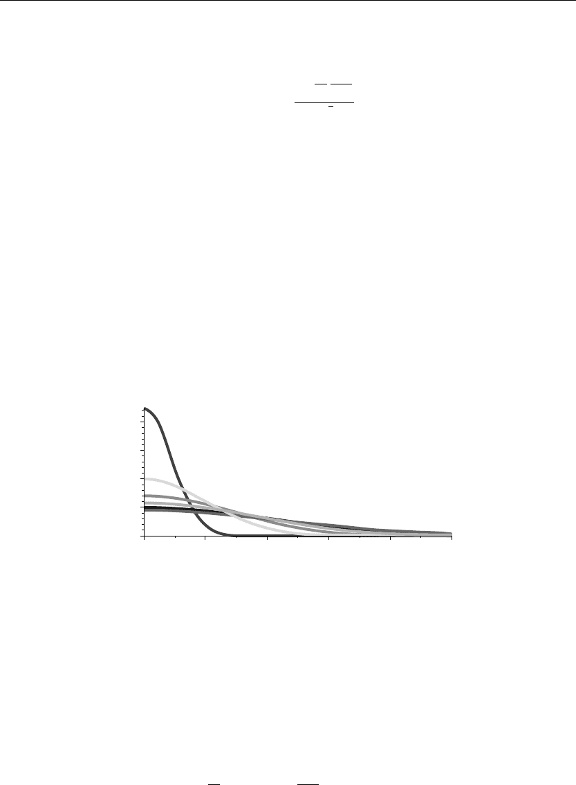
ANIMATION
> animate(u(x,t),x=0..1,t=0..5,thickness=3);
The preceding animation command shows the spatial-time temperature distribution u(x, t) in
the rod. The animation sequence here and in Figure 10.4 shows snapshots of the animation at
times t = 1/5, 1, 2, 3, 4, 5.
ANIMATION SEQUENCE
>u(x,0):=subs(t=1/5,u(x,t)):u(x,1):=subs(t=1,u(x,t)):
> u(x,2):=subs(t=2,u(x,t)):u(x,3):=subs(t=3,u(x,t)):
> u(x,4):=subs(t=4,u(x,t)):u(x,5):=subs(t=5,u(x,t)):
> plot({u(x,0),u(x,1),u(x,2),u(x,3),u(x,4),u(x,5)},x=0..10,thickness=10);
x~
0 0.2 0.4 0.6 0.8 1
0
0.5
1.0
1.5
2.0
Figure 10.4
EXAMPLE 10.5.6: (Input heat flux) We seek the temperature distribution u(x, t) in a thin rod
over the semi-infinite interval I ={x |0 <x<∞} whose lateral surface is insulated. The left
end of the rod has an input heat flux q(t) given following, and the initial temperature
distribution is 0. There is no internal heat source in the system, and the thermal diffusivity is
k = 1/20. We want to solve this problem using convolution methods.
SOLUTION: The diffusion partial differential equation is
∂
∂t
u(x, t) = k
∂
2
∂x
2
u(x, t)

660 Chapter 10
The boundary conditions are
u
x
(0,t)=−10 and u(∞,t)<∞
The initial condition is
u(x, 0) = 0
The Laplace transformed equation reads
∂
2
∂x
2
U(x, s) −
sU(x, s)
k
=−
f(x)
k
Here, U(x, s) is the Laplace transform of u(x, t) with respect to t. The transformed boundary
conditions are
∂
∂x
U(0,s)= Q(s) and U(∞,s)<∞
Assignment of system parameters
> restart:with(plots):with(inttrans):k:=1/20:q(t):=−10:f(x):=0:
Transformed equation in x reads
> diff(U(x,s),x,x)−(1/k)*s*U(x,s)=−1/k*f(x);
∂
2
∂x
2
U(x, s) −20sU(x, s) = 0 (10.55)
Transformed boundary conditions
> Q(s)=Int(q(t)*exp(−s*t),t=0..infinity);
Q(s) =
∞
0
−10 e
−st
dt (10.56)
> Q(s):=laplace(q(t),t,s);
Q(s) := −
10
s
(10.57)
General solution for U(x, s)
> assume(x>0):U(x,s):=C1(s)*exp(−sqrt(s/k)*x)+C2(s)*exp(sqrt(s/k)*x);
U(x∼,s):= C1(s) e
−2
√
5
√
sx∼
+C2(s) e
2
√
5
√
sx∼
(10.58)

Laplace Transform Methods for Partial Diff erential Equations 661
Substituting the boundary conditions at x = 0 and as x approaches infinity, for Re{s} > 0, we get
> C2(s):=0;
C2(s) := 0 (10.59)
> eq:=Q(s)=eval(subs(x=0,diff(U(x,s),x)));
eq := −
10
s
=−2C1(s)
√
5
√
s (10.60)
> C1(s):=solve(eq,C1(s));
C1(s) :=
√
5
s
3/2
(10.61)
Transformed solution
> U(x,s):=eval(U(x,s));
U(x∼,s):=
√
5e
−2
√
5
√
sx∼
s
3/2
(10.62)
Convolution partition
> U1(x,s):=U(x,s)*s;
U1(x∼,s):=
√
5e
−2
√
5
√
sx∼
√
s
(10.63)
> U2(x,s):=1/s;
U2(x∼,s):=
1
s
(10.64)
> u1(x,t):=invlaplace(U1(x,s),s,t);u1(x,tau):=subs(t=tau,u1(x,t)):
u1(x∼,t):=
√
5e
−
5x∼
2
t
√
πt
(10.65)
> u2(x,t):=simplify(invlaplace(U2(x,s),s,t));u2(x,t−tau):=subs(t=t−tau,u2(x,t)):
u2(x ∼,t):= 1 (10.66)
Convolution integral solution
> u(x,t):=Int(u1(x,tau)*u2(x,t−tau),tau=0..t);u(x,t):=simplify(value(%)):
u(x∼,t):=
t
0
√
5e
−
5x∼
2
τ
√
πτ
dτ (10.67)

662 Chapter 10
Conversion of integral to error function integral
> u(x,t):=simplify(convert(%,erfc));
u(x∼,t):=
2
−5
√
πx∼
√
t +
√
5e
−
5x∼
2
t
t +5x∼
√
π erf
√
5 x∼
√
t
√
t
√
π
√
t
(10.68)
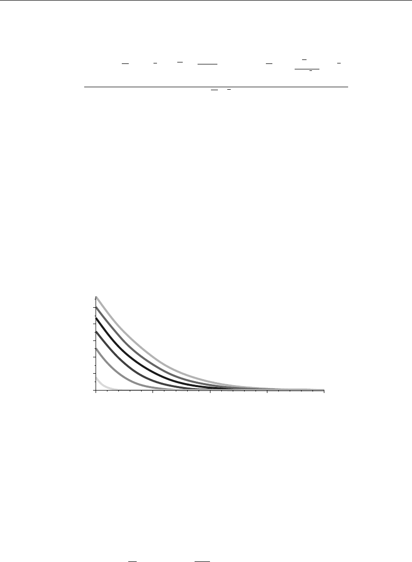
ANIMATION
> animate(u(x,t),x=0..2,t=1/10..5,thickness=3);
The preceding animation command shows the spatial-time temperature distribution u(x, t) in
the rod. The animation sequence here and in Figure 10.5 shows snapshots of the animation at
times t = 1/10, 1, 2, 3, 4, 5.
ANIMATION SEQUENCE
> u(x,0):=subs(t=1/10,u(x,t)):u(x,1):=subs(t=1,u(x,t)):
> u(x,2):=subs(t=2,u(x,t)):u(x,3):=subs(t=3,u(x,t)):
> u(x,4):=subs(t=4,u(x,t)):u(x,5):=subs(t=5,u(x,t)):
> plot({u(x,0),u(x,1),u(x,2),u(x,3),u(x,4),u(x,5)},x=0..2,thickness=10);
x~
0 0.5 1 1.5 2
0
1
2
3
4
5
Figure 10.5
EXAMPLE 10.5.7: (Rod with internal heat source) We seek the temperature distribution
u(x, t) in a thin rod over the semi-infinite interval I ={x |0 <x<∞} whose lateral surface is
insulated. The left end of the rod is held at the temperature 0, and the rod has an initial
temperature distribution of 0. There is an internal heat source h(x, t) in the system, given
following, and the thermal diffusivity is k = 1/5.
SOLUTION: The nonhomogeneous diffusion partial differential equation is
∂
∂t
u(x, t) = k
∂
2
∂x
2
u(x, t)
+h(x, t)

Laplace Transform Methods for Partial Diff erential Equations 663
The boundary conditions are
u(0,t)= 0 and u(∞,t)<∞
The initial condition is
u(x, 0) = 0
and the internal heat source is
h(x, t) = sin(x) e
−t
The Laplace transformed equation reads
∂
2
∂x
2
U(x, s) −
sU(x, s)
k
=−
f(x)
k
−
H(x, s)
k
Here, U(x, s) is the Laplace transform of u(x, t) with respect to t. The transformed boundary
conditions are
U(0,s)= Q(s) and U(∞,s)<∞
Assignment of system parameters
> restart:with(plots):with(inttrans):k:=1/5:q(t):=0:f(x):=0:h(x,t):=sin(x)*exp(−t):
Transformed boundary conditions
> Q(s):=Int(q(t)*exp(−s*t),t=0..infinity);
Q(s) :=
∞
0
0dt (10.69)
> Q(s):=laplace(q(t),t,s);
Q(s) := 0 (10.70)
Transformed heat source
> H(x,s):=Int(h(x,t)*exp(−s*t),t=0..infinity);
H(x, s) :=
∞
0
sin(x) e
−t
e
−st
dt (10.71)
> H(x,s):=laplace(h(x,t),t,s);H(v,s):=subs(x=v,H(x,s)):
H(x, s) :=
sin(x)
1 +s
(10.72)

664 Chapter 10
Transformed equation in x reads
> diff(U(x,s),x,x)−(1/k)*s*U(x,s)=−f(x)/k−H(x,s)/k;
∂
2
∂x
2
U(x, s) −5sU(x, s) =−
5 sin(x)
1 +s
(10.73)
Basis vectors to x equation
> phi[1](x,s):=exp(−sqrt(s/k)*x);phi[1](v,s):=subs(x=v,phi[1](x,s)):phi[2](x,s):
=exp(sqrt(s/k)*x);phi[2](v,s):=subs(x=v,phi[2](x,s)):
φ
1
(x, s) :=e
−
√
5
√
sx
φ
2
(x, s) :=e
√
5
√
sx
(10.74)
Evaluation of Wronskian
> W(phi[1](v,s),phi[2](v,s)):=simplify(phi[1](v,s)*diff(phi[2](v,s),v)−phi[2](v,s)*
diff(phi[1](v,s),v));
W
e
−
√
5
√
sv
, e
√
5
√
sv
:= 2
√
5
√
s (10.75)
Evaluation of Green’s function
> G(x,v,s):=(phi[1](v,s)*phi[2](x,s)−phi[1](x,s)*phi[2](v,s))/W(phi[1](v,s),phi[2](v,s));
G(x, v, s) :=
1
10
e
−
√
5
√
sv
e
√
5
√
sx
− e
−
√
5
√
sx
e
√
5
√
sv
√
5
√
s
(10.76)
Particular solution to the transformed equation
> Up(x,s):=−Int(G(x,v,s)*H(v,s)/k,v);Up(x,s):=value(%):
Up(x, s) := −
⎛
⎝
1
2
e
−
√
5
√
sv
e
√
5
√
sx
− e
−
√
5
√
sx
e
√
5
√
sv
√
5 sin(v)
√
s(1 +s)
dv
⎞
⎠
(10.77)
> Up(x,s):=simplify(subs(v=x,%));
Up(x, s) :=
5 sin(x)
(1 +s)(5s +1)
(10.78)

Laplace Transform Methods for Partial Diff erential Equations 665
General solution
> U(x,s):=C1(s)*phi[1](x,s)+C2(s)*phi[2](x,s)+Up(x,s);
U(x, s) := C1(s) e
−
√
5
√
sx
+C2(s) e
√
5
√
sx
+
5 sin(x)
(1 +s)(5s +1)
(10.79)
Substituting the boundary conditions at x = 0 and as x approaches infinity, for Re{s} > 0,
we get
> C2(s):=0;
C2(s) := 0 (10.80)
> eq:=Q(s)=eval(subs(x=0,U(x,s)));
eq := 0 = C1(s) (10.81)
> C1(s):=solve(eq,C1(s));
C1(s) := 0 (10.82)
Transformed solution
> U(x,s):=eval(U(x,s));
U(x, s) :=
5 sin(x)
(1 +s)(5s +1)
(10.83)
Final solution
> u(x,t):=invlaplace(U(x,s),s,t);
u(x, t) :=
5
2
sin(x) e
−
3
5
t
sinh
2
5
t
(10.84)
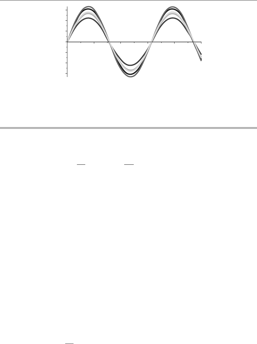
ANIMATION
> animate(u(x,t),x=0..10,t=0..5,thickness=3);
The preceding animation command shows the spatial-time temperature distribution u(x, t) in
the rod. The animation sequence here and in Figure 10.6 shows snapshots of the animation at
times t = 0, 1, 2, 3, 4, 5.
ANIMATION SEQUENCE
> u(x,0):=subs(t=0,u(x,t)):u(x,1):=subs(t=1,u(x,t)):
> u(x,2):=subs(t=2,u(x,t)):u(x,3):=subs(t=3,u(x,t)):
> u(x,4):=subs(t=4,u(x,t)):u(x,5):=subs(t=5,u(x,t)):
> plot({u(x,0),u(x,1),u(x,2),u(x,3),u(x,4),u(x,5)},x=0..10,thickness=10);

666 Chapter 10
x
0.6
0.4
0.2
0
2
0.2
24 8610
2
0.4
2
0.6
Figure 10.6
10.6 Laplace Transform Procedures on the
Wave Equation
We consider the nonhomogeneous partial differential equation for wave phenomena in one
spatial dimension in rectangular coordinates as given here:
∂
2
∂t
2
u(x, t) = c
2
∂
2
∂x
2
u(x, t)
+h(x, t)
with the two initial conditions
u(x, 0) = f(x) and u
t
(x, 0) = g(x)
The term h(x, t) accounts for any external sources in the system, f(x) denotes the initial
displacment distribution, and g(x) denotes the initial speed distribution. We assume that there
is no damping in the system.
In evaluating the Laplace transform of terms in the preceding equation, we have to contend
with taking improper integrals with respect to t of functions that are dependent on both x and t.
We denote the Laplace transform of u(x, t) with respect to the time variable t by the capital
letter representation as shown:
∞
0
u(x, t) e
−st
dt = U(x, s)
Proceeding formally with the evaluation of transforms of the derivative terms in the given
partial differential equation, we get
∞
0
∂
2
∂t
2
u(x, t)
e
−st
dt = s
2
U(x, s) −su(x, 0) −u
t
(x, 0)

Laplace Transform Methods for Partial Diff erential Equations 667
In the preceding, U(x, s) denotes the Laplace transform of u(x, t) with respect to t; u(x, 0)
denotes the initial value of u(x, t); and u
t
(x, 0) denotes the initial speed.
Proceeding formally, in evaluating the transforms of the partial derivative terms with respect to
the spatial variable x,weget
∞
0
∂
2
∂x
2
u(x, t)
e
−st
dt =
∂
2
∂x
2
U(x, s)
This operation assumes that we could interchange the order of the differentiation operation,
with respect to x, with the integration operation, with respect to t. The conditions for the
validity of doing this are based on the uniform convergence of the improper integrals of the
derivative terms.
Assuming the validity of all these given conditions, then the Laplace transform of the wave
partial differential equation gives us
∂
2
∂x
2
U(x, s) −
s
2
U(x, s)
c
2
=−
sf ( x )
c
2
−
g(x)
c
2
−
H(x, s)
c
2
Here, H(x, s) is the Laplace transform of the source term given as
H(x, s) =
∞
0
h(x, t) e
−st
dt
The preceding differential equation is an ordinary second-order nonhomogeneous differential
equation in the single spatial variable x. We investigated the solutions for this equation in
Chapter 1. The solutions are, of course, dependent on the spatial boundary conditions on the
problem.
We now implement the Laplace transform method to evaluate solutions to the wave equation
over semi-infinite domains with respect to the spatial variable x. We focus on those types of
problems that may or may not have nonhomogeneous boundary conditions—those problems
that cannot ordinarily be solved using Fourier transform methods as covered in Chapter 9.
Further, we do not consider using Laplace transform methods for wave problems over finite
domains here because eigenfunction expansion methods, as used in Chapters 4, 7, and 8, are
more effective.
In general, we consider time-dependent boundary conditions that are nonhomogeneous at
x = 0 and are bounded as x approaches infinity; that is,
κ
1
u(0,t)+κ
2
u
x
(0,t)= q(t)
and
u(∞,t)<∞
