Articolo G.A. Partial Differential Equations and Boundary Value Problems with Maple V
Подождите немного. Документ загружается.


648 Chapter 10
> Q(s):=laplace(q(t),t,s);
Q(s) :=
10
s
(10.4)
General solution for U(x, s)
> assume(x>0):U(x,s):=C1(s)*exp(−sqrt(s/k)*x)+C2(s)*exp(sqrt(s/k)*x);
U(x∼,s):= C1(s) e
−
√
10
√
sx∼
+C2(s) e
√
10
√
sx∼
(10.5)
Substituting the boundary conditions at x = 0 and as x approaches infinity, for Re{s} > 0, we get
> C2(s):=0;
C2(s) := 0 (10.6)
> eq:=Q(s)=eval(subs(x=0,U(x,s)));
eq :=
10
s
= C1(s) (10.7)
> C1(s):=solve(eq,C1(s));
C1(s) :=
10
s
(10.8)
Transformed solution
> U(x ,s):=eval(U(x,s));
U(x∼,s):=
10 e
−
√
10
√
sx∼
s
(10.9)
Solution is the inverse Laplace of U(x, s)
> u(x,t):=invlaplace(U(x,s),s,t);
u(x∼,t):= 10 erfc
1
2
x∼
√
10
√
t
(10.10)
ANIMATION
> animate(u(x,t),x=0..10,t=0..10,thickness=3);
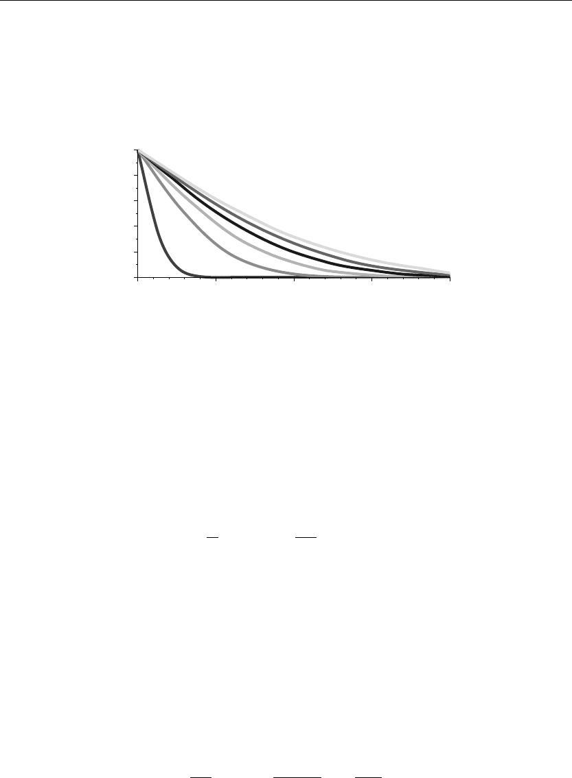
The preceding animation command shows the spatial-time temperature distribution u(x, t) in
the rod. The animation sequence shown here and in Figure 10.1 shows snapshots of the
animation at times t = 1/10, 1, 2, 3, 4, 5.
Laplace Transform Methods for Partial Diff erential Equations 649
ANIMATION SEQUENCE
> u(x,0):=subs(t=1/10,u(x,t)):u(x,1):=subs(t=1,u(x,t)):
> u(x,2):=subs(t=2,u(x,t)):u(x,3):=subs(t=3,u(x,t)):
> u(x,4):=subs(t=4,u(x,t)):u(x,5):=subs(t=5,u(x,t)):
> plot({u(x,0),u(x,1),u(x,2),u(x,3),u(x,4),u(x,5)},x=0..2,thickness=10);
x~
0 0.5 1 1.5 2
0
2
4
6
8
10
Figure 10.1
EXAMPLE 10.5.2: (Solution by convolution) We seek the temperature distribution u(x, t) in
a thin rod over the semi-infinite interval I ={x |0 <x<∞} whose lateral surface is insulated.
The left end of the rod has a temperature constraint u(0,t)= q(t) given following, and the
initial temperature distribution is 0. There is no internal heat source in the system and the
thermal diffusivity is k. We solve the problem by using the convolution method.
SOLUTION: The diffusion partial differential equation is
∂
∂t
u(x, t) = k
∂
2
∂x
2
u(x, t)
The boundary conditions are
u(0,t)= q(t) and u(∞,t)<∞
The initial condition is
u(x, 0) = 0
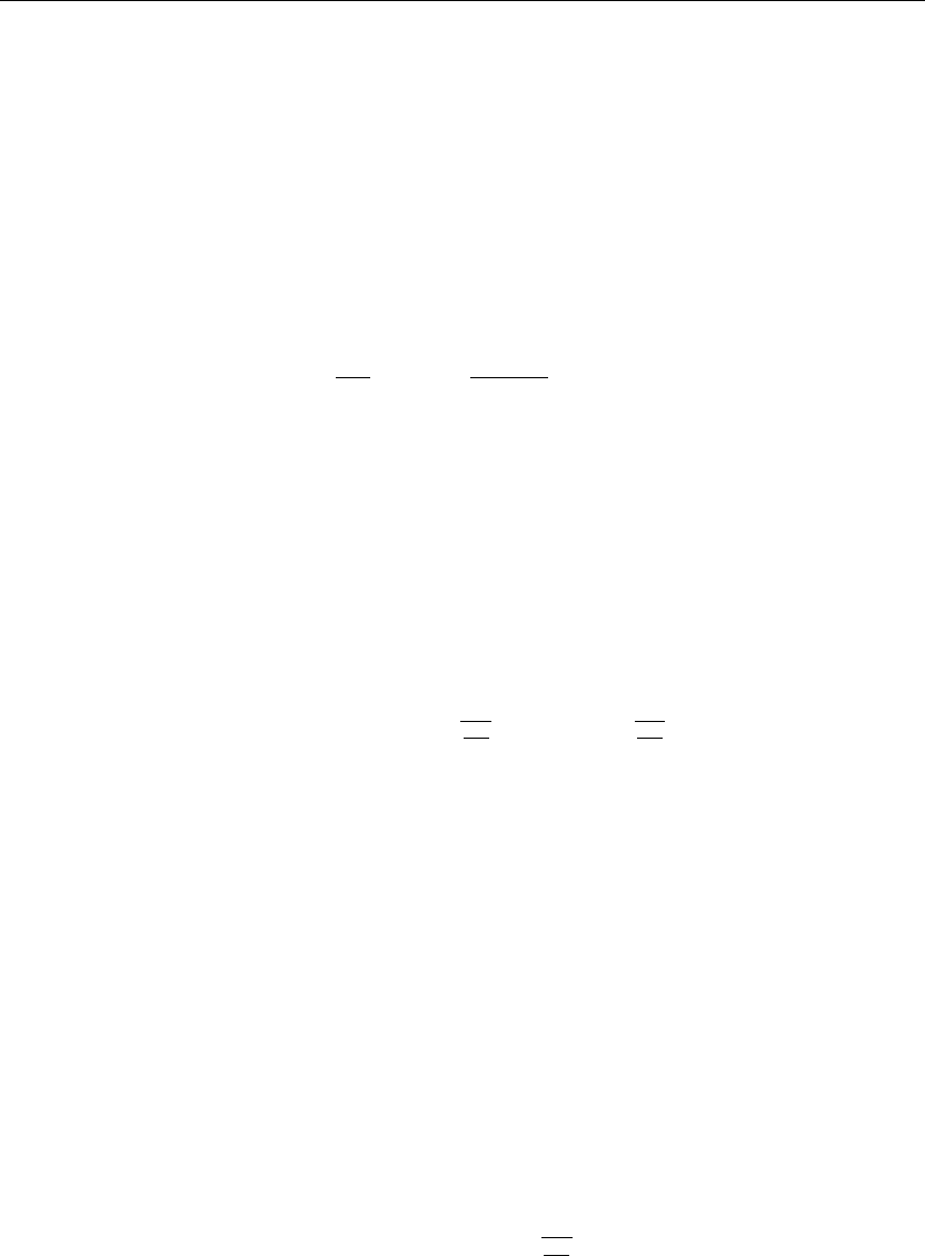
The Laplace transformed equation reads
∂
2
∂x
2
U(x, s) −
sU(x, s)
k
=−
f(x)
k
650 Chapter 10
Here, U(x, s) is the Laplace transform of u(x, t) with respect to t. The transformed boundary
conditions are
U(0,s)= Q(s) and U(∞,s)<∞
Assignment of system parameters
> restart:with(plots):with(inttrans):f(x):=0:
Transformed equation in x reads
> diff(U(x,s),x,x)−(1/k)*s*U(x,s)=−1/k*f(x);
∂
2
∂x
2
U(x, s) −
sU(x, s)
k
= 0 (10.11)
Transformed boundary conditions
> Q(s)=Int(q(t)*exp(−s*t),t=0..infinity);
Q(s) =
∞
0
q(t) e
−st
dt (10.12)
General solution for U(x, s)
> assume(x>0):assume(k>0):U(x,s):=C1(s)*exp(−sqrt(s/k)*x)+C2(s)*exp(sqrt(s/k)*x);
U(x∼,s):= C1(s) e
−
s
k∼
x∼
+C2(s) e
s
k∼
x∼
(10.13)
Substituting the boundary conditions at x = 0 and as x approaches infinity, for Re{s} > 0, we get
> C2(s):=0;
C2(s) := 0 (10.14)
> eq:=Q(s)=eval(subs(x=0,U(x,s)));
eq := Q(s) = C1(s) (10.15)
> C1(s):=solve(eq,C1(s));
C1(s) := Q(s) (10.16)
Transformed solution
> U(x,s):=eval(U(x,s));
U(x∼,s):= Q(s) e
−
s
k∼
x∼
(10.17)

Laplace Transform Methods for Partial Diff erential Equations 651
Convolution partition
> U1(x,s):=Q(s);
U1(x∼,s):= Q(s) (10.18)
> U2(x,s):=U(x,s)/Q(s);
U2(x∼,s):= e
−
s
k∼
x∼
(10.19)
> u1(x,t):=q(t);u1(x,tau):=subs(t=tau,u1(x,t)):
u1(x∼,t):= q(t) (10.20)
> u2(x,t):=simplify(invlaplace(U2(x,s),s,t));u2(x,t−tau):=subs(t=t−tau,u2(x,t)):
u2(x∼,t):=
1
2
x∼ e
−
1
4
x∼
2
k∼t
√
π
√
k∼t
3/2
(10.21)
Convolution integral solution
> u(x,t):=Int(u1(x,tau)*u2(x,t−tau),tau=0..t);u(x,t):=simplify(value(%)):
u(x∼,t):=
t
0
1
2
q(τ)x∼ e
−
1
4
x∼
2
k∼(t−τ)
√
π
√
k∼(t −τ)
3/2
dτ (10.22)
We leave the solution in the form of a convolution integral. This form of the solution can
accommodate any temperature constraint q(t) at x = 0. We leave specific cases for the
exercises.
EXAMPLE 10.5.3: We seek the temperature distribution u(x, t) in a thin rod over the
semi-infinite interval I ={x |0 <x<∞} whose lateral surface is insulated. The left end of the
rod is held at the temperature 0, and the rod has the initial temperature distribution f(x) given
following. There is no internal heat source in the system, and the thermal diffusivity is k = 1/5.
SOLUTION: The diffusion partial differential equation is
∂
∂t
u(x, t) = k
∂
2
∂x
2
u(x, t)
The boundary conditions are
u(0,t)= 0 and u(∞,t)<∞

652 Chapter 10
The initial condition is
u(x, 0) = sin(x)
The Laplace transformed equation reads
∂
2
∂x
2
U(x, s) −
sU(x, s)
k
=−
f(x)
k
Here, U(x, s) is the Laplace transform of u(x, t) with respect to t. The transformed boundary
conditions are
U(0,s)= Q(s) and U(∞,s)<∞
Assignment of system parameters
> restart:with(plots):with(inttrans):k:=1/5:q(t):=0:f(x):=sin(x):f(v):=subs(x=v,f(x)):
Transformed equation in x reads
> diff(U(x,s),x,x)−(1/k)*s*U(x,s)=−1/k*f(x);
∂
2
∂x
2
U(x, s) −5sU(x, s) =−5 sin(x) (10.23)
Transformed boundary conditions
> Q(s):=Int(q(t)*exp(−s*t),t=0..infinity);
Q(s) :=
∞
0
0dt (10.24)
> Q(s):=laplace(q(t),t,s);
Q(s) := 0 (10.25)
Basis vectors to x equation
> phi[1](x,s):=exp(−sqrt(s/k)*x);phi[1](v,s):=subs(x=v,phi[1](x,s)):phi[2](x,s)
:=exp(sqrt(s/k)*x);phi[2](v,s):=subs(x=v,phi[2](x,s)):
φ
1
(x, s) := e
−
√
5
√
sx
φ
2
(x, s) := e
√
5
√
sx
(10.26)

Laplace Transform Methods for Partial Diff erential Equations 653
Evaluation of Wronskian
> W(phi[1](v,s),phi[2](v,s)):=simplify(phi[1](v,s)*diff(phi[2](v,s),v)−phi[2](v,s)*
diff(phi[1](v,s),v));
W
e
−
√
5
√
sv
, e
√
5
√
sv
:= 2
√
5
√
s (10.27)
Evaluation of Green’s function
> G(x,v,s):=(phi[1](v,s)*phi[2](x,s)−phi[1](x,s)*phi[2](v,s))/W(phi[1](v,s),phi[2](v,s));
G(x, v, s) :=
1
10
e
−
√
5
√
sv
e
√
5
√
sx
− e
−
√
5
√
sx
e
√
5
√
sv
√
5
√
s
(10.28)
Particular solution to the transformed equation
> Up(x,s):=−Int(G(x,v,s)*f(v)/k,v);Up(x,s):=value(%):
Up(x, s) := −
⎛
⎝
1
2
e
−
√
5
√
sv
e
√
5
√
sx
− e
−
√
5
√
sx
e
√
5
√
sv
√
5 sin(v)
√
s
dv
⎞
⎠
(10.29)
> Up(x,s):=simplify(subs(v=x,%));
Up(x, s) :=
5 sin(x)
5s +1
(10.30)
General solution
> U(x,s):=C1(s)*phi[1](x,s)+C2(s)*phi[2](x,s)+Up(x,s);
U(x, s) := C1(s) e
−
√
5
√
sx
+C2(s) e
√
5
√
sx
+
5 sin(x)
5s +1
(10.31)
Substituting the boundary conditions at x = 0 and as x approaches infinity, for Re{s} > 0,
we get
> C2(s):=0;
C2(s) := 0 (10.32)
> eq:=Q(s)=eval(subs(x=0,U(x,s)));
eq := 0 = C1(s) (10.33)
> C1(s):=solve(eq,C1(s));
C1(s) := 0 (10.34)
654 Chapter 10
Transformed solution
> U(x,s):=eval(U(x,s));
U(x, s) :=
5 sin(x)
5s +1
(10.35)
Final solution
> u(x,t):=invlaplace(U(x,s),s,t);
u(x, t) := sin(x) e
−
1
5
t
(10.36)
ANIMATION
> animate(u(x,t),x=0..10,t=0..5,thickness=3);
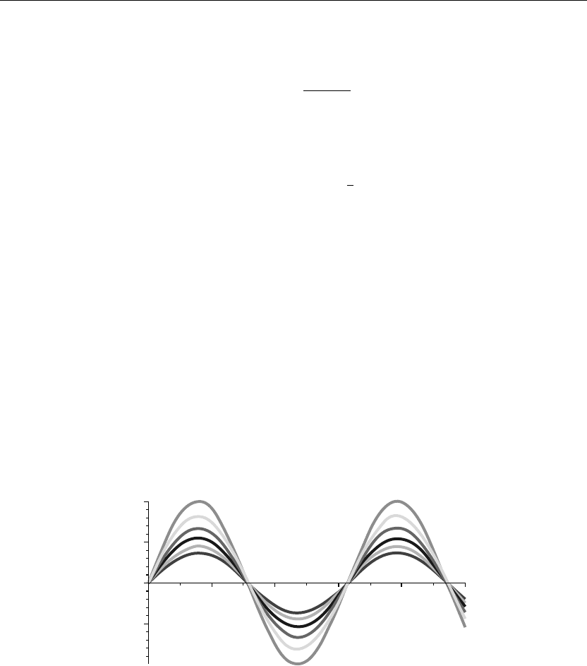
The preceding animation command shows the spatial-time temperature distribution u(x, t) in
the rod. The animation sequence here and in Figure 10.2 shows snapshots of the animation at
times t = 0, 1, 2, 3, 4, 5.
ANIMATION SEQUENCE
> u(x,0):=subs(t=0,u(x,t)):u(x,1):=subs(t=1,u(x,t)):
> u(x,2):=subs(t=2,u(x,t)):u(x,3):=subs(t=3,u(x,t)):
> u(x,4):=subs(t=4,u(x,t)):u(x,5):=subs(t=5,u(x,t)):
> plot({u(x,0),u(x,1),u(x,2),u(x,3),u(x,4),u(x,5)},x=0..10,thickness=10);
x
246810
2
0.5
0
0.5
1.0
Figure 10.2
EXAMPLE 10.5.4: (Applied Dirac delta function) We seek the temperature distribution
u(x, t) in a thin rod over the interval I ={x |0 <x<∞} whose lateral surface is insulated. The
left end of the rod has an applied impulse temperature (Dirac delta function). The rod has an
initial temperature distribution u(x, 0) = 0, and there are no internal heat sources in the system.
The thermal diffusivity is k = 1.

Laplace Transform Methods for Partial Diff erential Equations 655
SOLUTION: The diffusion partial differential equation is
∂
∂t
u(x, t) = k
∂
2
∂x
2
u(x, t)
The boundary conditions are
u(0,t)= δ(t) and u(∞,t)<∞
The initial condition is
u(x, 0) = 0
The Laplace transformed equation reads
∂
2
∂x
2
U(x, s) −
sU(x, s)
k
=−
f(x)
k
Here, U(x, s) is the Laplace transform of u(x, t) with respect to t. The transformed boundary
conditions are
U(0,s)= Q(s) and U(∞,s)<∞
Assignment of system parameters
> restart:with(plots):with(inttrans):k:=1:q(t):=Dirac(t):f(x):=0:
Transformed equation in x reads
> diff(U(x,s),x,x)−(1/k)*s*U(x,s)=−1/k*f(x);
∂
2
∂x
2
U(x, s) −sU(x, s) = 0 (10.37)
Transformed boundary conditions
> Q(s):=Int(q(t)*exp(−s*t),t=0..infinity);
Q(s) :=
∞
0
Dirac(t) e
−st
dt (10.38)
> Q(s):=laplace(q(t),t,s);
Q(s) := 1 (10.39)

656 Chapter 10
General solution for U(x, s)
> assume(x>0):U(x,s):=C1(s)*exp(−sqrt(s/k)*x)+C2(s)*exp(sqrt(s/k)*x);
U(x∼,s):= C1(s) e
−
√
sx∼
+C2(s) e
√
sx∼
(10.40)
Substituting the boundary conditions at x = 0 and as x approaches infinity, for Re{s} > 0,
we get
> C2(s):=0;
C2(s) := 0 (10.41)
> eq:=Q(s)=eval(subs(x=0,U(x,s)));
eq := 1 = C1(s) (10.42)
> C1(s):=solve(eq,C1(s));
C1(s) := 1 (10.43)
Transformed solution
> U(x,s):=eval(U(x,s));
U(x∼,s):= e
−
√
sx∼
(10.44)
Solution is the inverse Laplace of U(x, s)
> u(x,t):=invlaplace(U(x,s),s,t);
u(x∼,t):=
1
2
x∼ e
−
1
4
x∼
2
t
√
πt
3/2
(10.45)
ANIMATION
> animate(u(x,t),x=0..10,t=0..5,thickness=3);
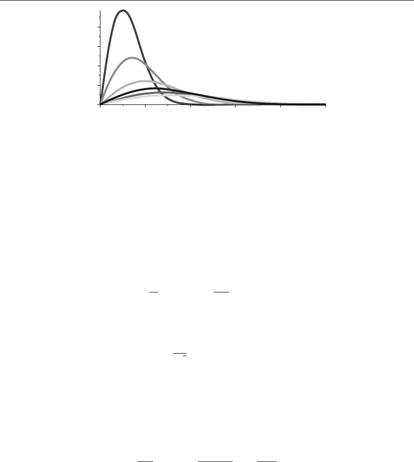
The preceding animation command shows the spatial-time temperature distribution u(x, t) in
the rod. The animation sequence here and in Figure 10.3 shows snapshots of the animation at
times t = 1/2, 1, 2, 3, 4, 5.
ANIMATION SEQUENCE
> u(x,0):=subs(t=1/2,u(x,t)):u(x,1):=subs(t=1,u(x,t)):
> u(x,2):=subs(t=2,u(x,t)):u(x,3):=subs(t=3,u(x,t)):
> u(x,4):=subs(t=4,u(x,t)):u(x,5):=subs(t=5,u(x,t)):
> plot({u(x,0),u(x,1),u(x,2),u(x,3),u(x,4),u(x,5)},x=0..10,thickness=10);
Laplace Transform Methods for Partial Diff erential Equations 657
x~
0246810
0
0.1
0.2
0.3
0.4
Figure 10.3
EXAMPLE 10.5.5: (End of rod with temperature constraint) We seek the temperature
distribution u(x, t) in a thin rod over the interval I ={x |0 <x<∞} whose lateral surface is
insulated. The left end of the rod is constrained at a varying temperature q(t) given following,
and the rod has an initial temperature distribution u(x, 0) = 0. There is no heat source in the
system and the thermal diffusivity of the rod is k = 1/50.
SOLUTION: The diffusion partial differential equation is
∂
∂t
u(x, t) = k
∂
2
∂x
2
u(x, t)
The boundary conditions are
u(0,t)=
1
√
t
and u(∞,t)<∞
The initial condition is
u(x, 0) = 0
The Laplace transformed equation reads
∂
2
∂x
2
U(x, s) −
sU(x, s)
k
=−
f(x)
k
Here, U(x, s) is the Laplace transform of u(x, t) with respect to t. The transformed boundary
conditions are
U(0,s)= Q(s) and U(∞,s)<∞
Assignment of system parameters
> restart:with(plots):with(inttrans):k:=1/50:q(t):=1/sqrt(t):f(x):=0:
