Alexandrov A.S.,Theory of Superconductivity - From Weak to Strong Coupling

Подождите немного. Документ загружается.

Intermediate-coupling theory

is the Fourier transform of the second derivative of the ion potential energy. The

ﬁrst derivative in equation (3.6) is zero in crystals with a centre of symmetry.

Different solutions of equation (3.12) are classiﬁed with the phonon branch

(mode) quantum number ν, which is 1, 2, 3 for a simple lattice and 1,...,3k

for a lattice with k ions per unit cell.

The periodic part of the Hamiltonian H

is diagonal in the Bloch

representation (appendix A):



(r) =



k,n,s

nks

(r)c

nks

(3.15)

where c

nks

are the fermion annihilation operators. The Bloch function obeys the

Schr¨odinger equation



−

∇

+ V (r)



nks

(r) = E

nks

(r). (3.16)

One-particle states are sorted with the momentum k in the Brillouin zone, band

index n and spin s. The solutions of this equation allow us to calculate the periodic

electron density n

(0)

(r), which determines the crystal ﬁeld potential V (r).The

LDA can explain the shape of the Fermi surface of wide-band metals and gaps

in narrow-gap semiconductors. The spin-polarized version of LDA can explain a

variety of properties of many magnetic materials. This is not the case in narrow

d- and f-band metals and oxides (and other ionic lattices), where the electron–

phonon interaction and Coulomb correlations are strong. These materials display

much less band dispersion and wider gaps compared with the ﬁrst-principle band

structure calculations. Using the phonon and electron annihilation and creation

operators, the Hamiltonian is written as

H = H

+ H

e−ph

+ H

e−e

(3.17)

where



k,n,s

nks

†

nks



q,ν

qν

†

qν

+ 1/2) (3.18)

describes independent Bloch electrons and phonons, ξ

nks

= E

nks

−µ is the band

energy spectrum with respect to the chemical potential. The part of the electron–

phonon interaction, which is linear in phonon operators, can be written as

e−ph

√



k,q,n,n



,ν,s



(q, k,ν)ω

qν

†

nks

nk−qs

qν

+ H.c. (3.19)

where



(q, k,ν) =−

1/2

3/2

qν



dr (e

qν

· ∇v(r))ψ

∗

nks

(r)ψ



k−qs

(r) (3.20)

Phonons in metal

is the dimensionless matrix element. Low-energy physics is often described by a

single-band approximation with the matrix element γ

(q, k,ν) depending only

on the momentum transfer q (the Fr¨ohlich interaction):



(q, k,ν) = γ(q,ν). (3.21)

The terms of H

e−ph

which are quadratic and higher orders in the phonon operators

are small. They have a role to play only for those phonons which are not coupled

with electrons by the linear interaction (3.20). The electron–electron correlation

energy of a homogeneous electron system is often written as

e−e



(q)ρ

†

(3.22)

where V

(q) is a matrix element, which is zero for q = 0 because of

electroneutrality and

†



k,s

†

k+qs

(3.23)

is the density ﬂuctuation operator. H

should also include a random potential in

doped semiconductors and amorphous metals.

3.2 Phonons in metal

In wide-band metals such as Na or K, the correlation energy is relatively small

≤ 1) and carriers are almost free. Core electrons together with nuclei form

compact ions with an effective Z . The carrier wavefunction outside the core can

be approximated by a plane wave

nks

(r)  e

ik·r

(3.24)

and the carrier density n

(0)

(r) is a constant. Therefore, the only relevant

interaction in the dynamic matrix (equation (3.7)) is the Coulomb repulsion

between ions, which yields

αβ

(l − m) =

∂

∂l

∂m





=m



− m



. (3.25)

The electron–ion interaction is a pure Coulomb attraction v(r) =−Ze

/r, which

is expanded in the Fourier series as

= 4π lim

κ→0



+ κ

iq·r

. (3.26)

Substituting this expansion into equations (3.25) and (3.20), we obtain

αβ

(m) = 4π lim

κ→0



+ κ

cos(q · m) (3.27)

Intermediate-coupling theory

+ +

= +

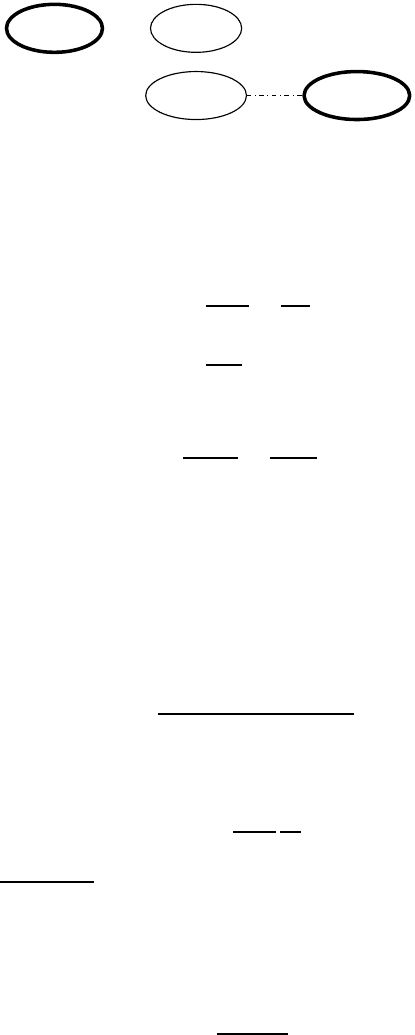
D(q,ω)

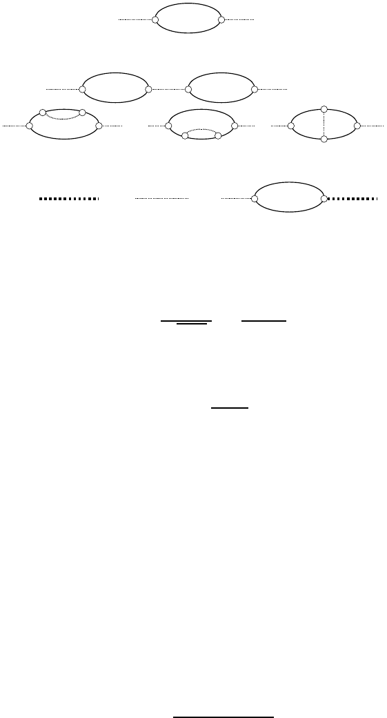
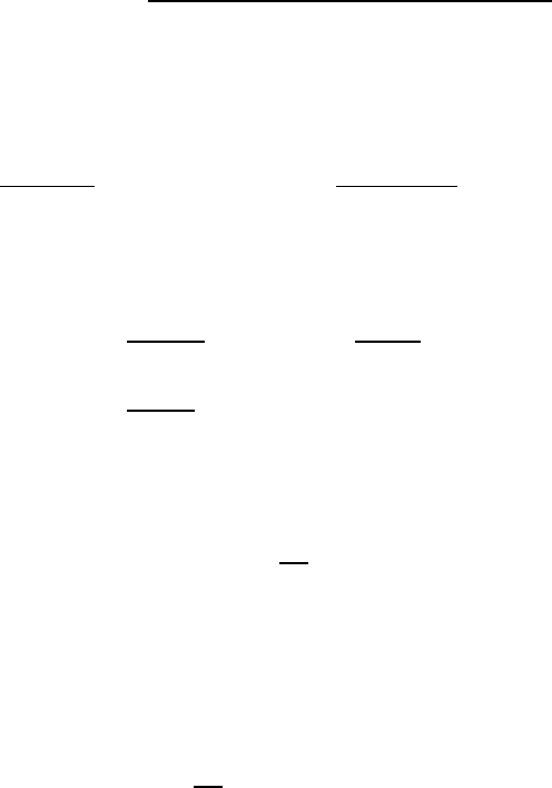
Figure 3.1. Second (a) and fourth order (b), (c), (d), (e) corrections to the phonon GF. The

phonon GF in the Migdal approximation (f ).

and

γ(q,ν) = i

4π NZe



Mω

lim

κ→0

qν

· q

+ κ

. (3.28)

Calculating the Fourier transform of equation (3.27), one obtains the following

equation for phonon frequencies and polarization vectors:

qν

= ω

qν

· q

. (3.29)

A longitudinal mode with e  q is the ion plasmon

= ω

(3.30)

and two shear (transverse) modes with e ⊥ q have zero frequencies, which is

the result of our approximation considering ions as rigid charges. In fact, core

electrons undergo a polarization, when ions are displaced from their equilibrium

positions, which yields a ﬁnite shear mode frequency.

According to equation (3.28), the carriers interact only with longitudinal

phonons. The interaction gives rise to a signiﬁcant renormalization of the

bare phonon frequency (equation (3.30)). We apply the Green’s function (GF)

formalism (appendix D) to calculate the renormalized phonon frequency. The

Fourier component of the free-electron GF is given by equation (2.163) with

= k

/2m

−µ. For interacting electrons, the electron self-energy is introduced

(k,ω) =[G

(0)

(k,ω)]

−1

−[G(k,ω)]

−1

(3.31)

and

G(k,ω) =

ω − ξ

− (k,ω)

. (3.32)

Phonons in metal

The phonon GF is deﬁned as

D(q, t) =−i

T

(t)d

†

+ d

†

(t)d

), (3.33)

and its Fourier transform for free phonons is a dimensionless even function of

frequency,

(0)

(q,ω) =

− ω

+ iδ

. (3.34)

The phonon self-energy is

(q,ω) =[D

(0)

(q,ω)]

−1

−[D(q,ω)]

−1

. (3.35)

The Feynman diagram technique is convenient, see ﬁgure 3.1. Thin straight

and dotted lines correspond to G

(0)

and D

(0)

, respectively, a vertex (circle)

corresponds to the interaction matrix element γ(q)



/N and bold lines

represent G and D.TheFr¨ohlich interaction is the sum of two operators

describing the emission and absorption of a phonon. Both events are taken into

account in the deﬁnition of D. Therefore wavy lines have no direction. There are

no ﬁrst- or higher-odd orders corrections to D because the Fr¨ohlich interaction is

off-diagonal with respect to phonon occupation numbers. The second-order term

in D (ﬁgure 3.1(a)) includes the so-called polarization bubble, 

(0)

,whichisa

convolution of two G

(0)

. Among different fourth-order diagrams the diagram in

ﬁgure 3.1(b) with two polarization loops is the most ‘dangerous’ one. Differing

from others, it is proportional to 1/q

, which is large for small q.However,the

singularity of internal vertices is ‘integrated out’ in the diagrams in ﬁgures 3.1(c)–

(d). The sum of all dangerous diagrams is given in ﬁgure 3.1(f )whichis

(q,ω) =

|γ(q)|



(q,ω) (3.36)

where



(q,ω) = 

(0)

(q,ω) (3.37)

and



(0)

(q,ω) =−

(2π)



dk d G

(0)

(k + q, + ω)G

(0)

(k,). (3.38)

The additional factor 2 in the phonon self-energy is due to a contribution of two

electron spin states. It is convenient to integrate over frequency in equation (3.38)

ﬁrst with the following result:



(0)

(q,ω) =

4π



(ξ

) − (ξ

k+q

)

ω + ξ

− ξ

k+q

+ iδ sign(ξ

k+q

)

. (3.39)

Intermediate-coupling theory



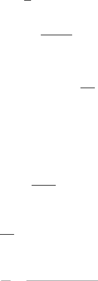
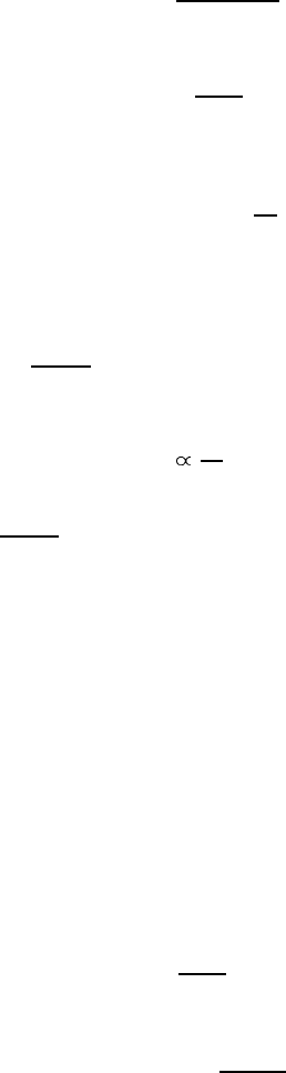
πH



T



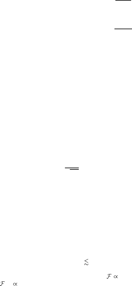
Figure 3.2. Screened polarization bubble 

(q,ω).

The phonon frequency ω is small, ω  µ. Thus, we can take the limit ω → 0in



(0)

and obtain

Re 

(q,ω) =−

2π





(3.40)

Im 

(q,ω) =−

2πq

|ω|(2k

− q) (3.41)

where

h(x ) = 1 +

1 − x



1 + x

1 − x



We should also take the Coulomb electron–electron interaction into account

because the corresponding vertex is singular in the long-wavelength limit,

(q) = 4πe

. This leads to a drastic renormalization of the long wave-

length behaviour of 

. In the ‘bubble’ or random phase approximation (RPA),

we obtain ﬁgure 3.2 as in the case of the electron–ion plasmon interaction,

ﬁgure 3.1(f ), but with the Coulomb (dashed-dotted) line instead of the dotted

phonon line. In the analytical form, we have



(q,ω) =



(0)

(q,ω)

1 − (4πe

)

(q,ω)

. (3.42)

As a result, in the long-wavelength limit q  q

one obtains



(q,ω) =−

(3.43)

where q



/π is the inverse (Debye) screening radius.

While 

(0)

is ﬁnite at q → 0, the screened 

(q,ω) iszerointhis

limit. Using the RPA expressions (equations (3.40)–(3.42)) and γ

determined

in equation (3.28) for ω

= ω

, we obtain the phonon GF as

D(q,ω) =

−˜ω

. (3.44)

Electrons in metal

The poles of D determine a new phonon dispersion and a damping  due to

interaction with electrons:

˜ω

(q, ˜ω

)

1/2

(3.45)

where

(q,ω) = 1 −

4πe



(0)

(q,ω) (3.46)

is the electron dielectric function. In the long-wavelength limit,

(q, 0) = 1 +

(3.47)

and we obtain the sound wave as the real part of ˜ω:

˜ω

= sq (3.48)

where s = Zk

√

3Mm

is the sound velocity. The imaginary part of ˜ω

determines the damping of the sound,



˜ω. (3.49)

Because the ratio of the sound velocity to the Fermi velocity (v

) is adiabatically

small (s/v



√

/M), the damping is small ( ˜ω). Electrons screen the

bare ion–ion Coulomb repulsion and the residual short-range dynamic matrix has

the sound-wave linear dispersion of the eigenfrequencies in the long-wavelength

limit.

3.3 Electrons in metal

The lowest contribution to the electron self-energy is given by two second-order

diagrams, see ﬁgures 3.3(a)and(b). The diagram in ﬁgure 3.3(b) is proportional

to |γ(q)|

with q ≡ 0, which is zero according to equation (3.28).

Higher-order diagrams are taken into account by replacing the bare ionic

plasmon GF by a renormalized one, equation (3.44), and the bare electron–

phonon interaction γ(q) by a screened one, γ

(q,ω), as shown in ﬁgure 3.4.

Presented analytically, the diagram in ﬁgure 3.4 corresponds to

(q,ω) = γ(q) +

4πe



(0)

(q,ω)γ

(q,ω) (3.50)

so that

(q,ω) =

γ(q)

(q,ω)

. (3.51)

Intermediate-coupling theory

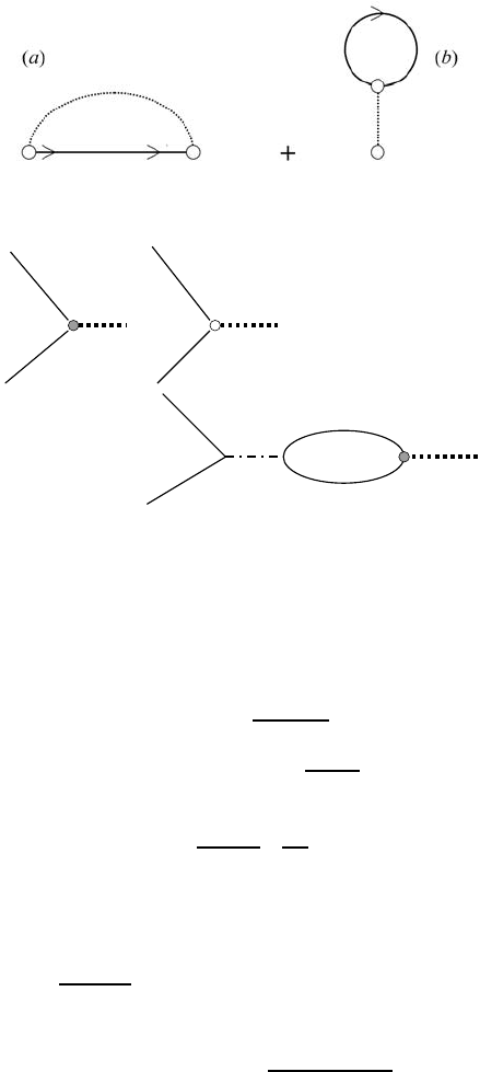
Figure 3.3. Second-order electron self-energy.



Figure 3.4. Screened electron–phonon interaction (dark circle).

For low-energy excitations (ω  µ) a static approximation of the dielectric

function (3.47) is appropriate. Instead of the D and γ

given by equations (3.44)

and (3.51), respectively, we introduce the acoustic phonon GF

D(q,ω) =

˜ω

−˜ω

(3.52)

and the electron–acoustic phonon vertex ˜γ(q)



˜ω

/N ,where

˜γ(q) =

γ(q)

(q, 0)



˜ω



3/2

. (3.53)

Finally we obtain the diagram in ﬁgure 3.5 for the electron self-energy as a

result of the summation of the most divergent diagrams, which is

(k,) =

(2π)



dq dω E

G(k − q, −ω)

D(q,ω) (3.54)

where

=|˜γ(q)|

˜ω

2µ

Z(1 +q

)

. (3.55)

Because Z is of the order of one, the electron–acoustic phonon interaction

is generally of the order of the Fermi energy. Therefore, one has to consider

Electrons in metal

Figure 3.5. Electron self-energy in the Migdal approximation.

Figure 3.6. Adiabatically small corrections to the electron self-energy.

fourth- and higher-order diagrams with the crossing phonon lines as in ﬁgure 3.6,

which are absent in ﬁgure 3.5. These diagrams are known as vertex corrections.

Fortunately, as shown by Migdal [48], their contribution is adiabatically small

(∼s/v

) compared with equation (3.54). This result is known as Migdal’s

‘theorem’.

The electron energy spectrum, renormalized by the electron–phonon

interaction, is determined as the pole of the electron GF,

≡

−˜µ = v

(k − k

) + δE

(3.56)

where

δ E

= (k,

) − (k

, 0) (3.57)

and ˜µ = µ + (k

, 0) is the renormalized Fermi energy. The region of large

q  k

 q

contributes mostly to the integral in equation (3.54). The

dimensionless coupling constant λ = 2E

N(E

) is small in this region,

λ ≈ r

 1 (3.58)

and the second order is sufﬁcient in our calculations of . Hence, we can

replace the exact GF in the integral equation (3.54) by the free GF. This is

appropriate for almost all quasi-particle energies. The difference between G and

(0)

appears to be important only for the damping calculations in a very narrow

region |

|ω

s/v

near the Fermi surface. As a result, we obtain

δ E

2iE

(2π)



dq dω

D(q,ω)[G

(0)

(k − q,

− ω) − G

(0)

− q, −ω)].

(3.59)

To simplify the calculations, we take E

as a constant and apply the Debye

approximation ˜ω

= sq for q < q

where q

 π/a is the Debye momentum.

We also consider a half-ﬁlled band, k

≈ π/2a with the energy-independent DOS

near the Fermi level N(E

) = m

/4π.

The main contribution to the integral in equation (3.59) comes from the

momentum region close to the Fermi surface,

|k − q|k

. (3.60)

Intermediate-coupling theory

It is convenient to introduce a new variable k



=|k − q| instead of the angle 

between k and q, and extend the integration to ±∞ for ξ = v



− k

).Then

the angular integration in equation (3.59) yields



d sin (...)∼



∞

−∞

dξ

[

ξ − ω − ξ + iδ sign(ξ)][ω + ξ − iδ sign(ξ)]

(3.61)

This integral is non-zero only if

ξ>ω>0or

ξ<ω<0. It is −2πiinthe

ﬁrst region and 2πi in the second region. Taking into account that

D is an even

function of ω, we obtain

δ E

(2π)



dqq



ξ|

dω sign(

ξ)

˜ω

−˜ω

+ iδ

. (3.62)

The real and imaginary parts of equation (3.62) determine the renormalized

spectrum and the lifetime of quasi-particles, respectively:

Re(δ E

) =

4π



dqq˜ω



˜ω

−

˜ω



(3.63)

Im(δE

) =

4πv



dqq˜ω

sign(

ξ) (3.64)

with q

ξ|/s if |

ξ| <ω

and q

= q

if |

ξ| >ω

. For excitations far away

from the Fermi surface (|

ξ|ω

),weﬁnd

Re(δ E

) =−λ

(3.65)

and for low-energy excitations with |

ξ|ω

Re(δ E

) =−λ

ξ. (3.66)

This means an increase in the effective mass of the electron due to the electron–

phonon interaction,

ξ =

∗

(k − k

) (3.67)

where the renormalized mass is

∗

= (1 + λ)m

. (3.68)

Hence, the excitation spectrum of metals has two different regions with two

different values of the effective mass. The thermodynamic properties of a metal at

low temperatures T  ω

involve m

∗

but the optical properties in the frequency

range ν  ω

are determined by high-energy excitations, where, according to

equation (3.65), corrections are small and the mass is equal to the band mass m

Eliashberg equations

Damping shows just the opposite behaviour. The integral in equation (3.64),

yields

Im(δE

) = sign(

ξ)

πλω

(3.69)

if |

ξ| >ω

and

Im(δ E

) = sign(

ξ)

πλ|

ξ|

3ω

(3.70)

if |

ξ|ω

These expressions describe the rate of decay of quasi-particles due to the

emission of phonons. In the immediate neighbourhood of the Fermi surface,

ξ|ω

, the decay is small compared with the quasi-particle energy |

ξ| even for

a relatively strong coupling λ ∼ 1 and the concept of well-deﬁned quasi-particles

has a deﬁnite meaning. Within the Migdal approximation the electron–phonon

interaction does not destroy the Fermi-liquid behaviour of electrons. The Pauli

exclusion principle is responsible for the stability of the Fermi liquid. In the

intermediate-energy region |

ξ|∼ω

, the decay is comparable with the energy

and the quasi-particle spectrum loses its meaning. In the high-energy region

ξ|ω

, the decay becomes small again in comparison with |

ξ| and the quasi-

particle concept recovers its meaning.

Going beyond the Migdal approximation, we have to consider adiabatically

small higher-order diagrams, that is to solve the Hamiltonian of free electrons and

acoustic phonons coupled by an interaction:

e−ph

√



k,q,s

˜γ(q) ˜ω

†

k−qs

+ H.c. (3.71)

where

is the acoustic-phonon annihilation operator. From our consideration,

it follows that, in applying this Hamiltonian to electrons, one should not consider

the acoustic phonon self-energy. Acoustic phonons in a metal appear as a result

of the electron-plasmon coupling and the Coulomb screening, so their frequency

already includes the self-energy effect (section 3.2).

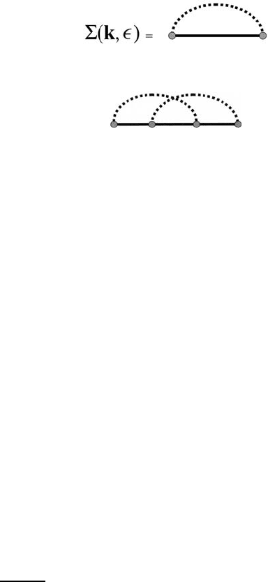
3.4 Eliashberg equations

Based on Migdal’s theorem, Eliashberg [36] extended BCS theory towards the

intermediate-coupling regime (λ

1), applying the Gor’kov formalism. The

condensed state is described by a classical ﬁeld, which is the average of the

product of two annihilation ﬁeld operators

ψψ or two creation operators

ψ

†

. These averages are macroscopically large below T

.The

appearance of anomalous averages cannot be seen perturbatively but they should

be included in the self-energy diagram, ﬁgure 3.5, from the very beginning. This