White R.E. Computational Mathematics: Models, Methods, and Analysis with MATLAB and MPI

Подождите немного. Документ загружается.

4.1. NONLINEAR PROBLEMS IN ONE VARIABLE 149

Table 4.1.1: Quadratic Convergence

m x

@(E

p1

)

0 1.0 0.414213

1 1.5 0.085786 2.000005

2 1.4166666 0.002453 3.000097

3 1.4142156 0.000002 3.008604

Table 4.1.2: Local Convergence

m for conv. x

m for conv.

10.0 no conv. 00.1 4

05.0 no conv. -0.5 6

04.0 6 -0.8 8

03.0 5 -0.9 20

01.8 3 -1.0 no conv.

iterates are computed in the loop given by lines 4-9. The algorithm is stopped

in lines 6-8 when the di

erence between two iterates is less than .0001.

MATLAB Codes picard.m and gpic.m

1. clear;

2. x(1) = 1.0;

3. eps = .0001;

4. for m=1:20

5. x(m+1) = gpic(x(m));

6. if abs(x(m+1)-x(m))

?eps

7. break;

8. end

9. end

10. x’

11. m

12. ﬁxed_point = x(m+1)

function gpic = gpic(x)

gpic = 1. + 1.0*(x/(1. + x));

Output from picard.m:

ans =

1.0000

1.5000

1.6000

1.6154

1.6176

1.6180

150 CHAPTER 4. NONLINEAR AND 3D MODELS

m =

ﬁxed_point =

1.6180

The M

AT LAB ﬁle newton.m contains the Newton algorithm for solving the

root problem 0 = 2

 {

, which is deﬁned in the function ﬁle fnewt.m. The

iterates are computed in the loop given by lines 4-9. The algorithm is stopped in

lines 6-8 when the residual

i({

) is less than .0001. The numerical results are

method. A similar code is newton.f90 written in Fortran 9x.

MATLAB Codes newton.m, fnewt.m and fnewtp.m

1. clear;

2. x(1) = 1.0;

3. eps = .0001;

4. for m=1:20

5. x(m+1) = x(m) - fnewt(x(m))/fnewtp(x(m));

6. if abs(fnewt(x(m+1)))

?eps

7. break;

8. end

9. end

10. x’

11. m

12. ﬁxed_point = x(m+1)

function fnewt = fnewt(x)

fnewt =2 - x^2;

function fnewtp = fnewtp(x)

fnewtp = -2*x;

4.1.6 Assessment

In the radiative cooling mod el we have also ignored the good possibility that

there will be di

erences in temperature according to the location in space. In

such cases there will be diusion of heat, and one must model this mode of heat

transfer.

We indicated that the Picard algorithm may converge if the mapping

j({)

is contractive. The following theorem makes this more precise. Under some

additional assumptions the new error is bounded by the old error.

Theorem 4.1.1 (Picard Convergence) Let g:[a,b]

$[a,b] and assume that x is

a ﬁxed point of g and x is in [a,b]. If g is contractive on [a,b], then the Picard

algorithm in (4.1.2) converges to the ﬁxed point. Moreover, the ﬁxed point is

unique.

in Table 4.4.1 where convergence is obtained after three iterations on Newton’s

4.1. NONLINEAR PROBLEMS IN ONE VARIABLE 151

Proof. Let

{

p+1

= j({

) and { = j({). Repeatedly use the contraction

property (4.1.4).

{

p+1

 {| = |j({

)  j({)|

 u|{

 {|

u|j({

p1

)  j({)|

 u

p2

 {|

 u

p+1

 {|= (4.1.9)

Since 0

 u ? 1> u

p+1

must go to zero as m increases.

If there is a second ﬁxed point

|, then |{  || = |j({)  j(|)|  u||  {|

where

u ? 1. So, if { and | are dierent, then ||  {| is not zero. Divide both

sides by |

|  {| to get 1  u, which is a contradiction to our assumption that

u ? 1. Evidently, { = |=

In the above examples we noted that Newton’s algorithm was a special case

of the Picard algorithm with j({) = {  i({)@i

({). In order to show j({) is

contractive, we need to have, as in (4.1.6), |

({)| ? 1.

({) = 1  (i

({)

 i({)i

({))@i

({)

= i({)i

({)@i

({)

(4.1.10)

If b

{ is a solution of i({) = 0 and i({) is continuous, then we can make i({)

as small as we wish by choosing

{ close to b{. So, if i

({)@i

({)

is bounded,

then j({) will be contractive for { near b{. Under the conditions listed in the

following theorem this establishes the local convergence.

Theorem 4.1.2 (Newton’s Convergence) Consider

i({) = 0 and assume b{ is

a root. If

(b{) is not zero and i

({) is continuous on an interval containing

{, then

1. Newton’s algorithm converges locally to the b

{, that is, for {

suitably close

to b{ and

2. Newton’s algorithm converges quadratically, that is,

p+1

 b{|  [pd{|i

({)|@(2 plq|i

({)|]|{

 b{|

= (4.1.11)

Proof. In order to prove the quadratic convergence, use the extended mean

value theorem where

d = {

and { = b{ to conclude that there is some c such

that

0 =

i(b{) = i({

) + i

({

)(b{  {

) + (i

(f)@2)(b{  {

)

Divide the above by i

({

) and use the deﬁnition of {

p+1

0 = ({

p+1

 {

) + (b{  {

) + (i

(f)@(2i

({

))(b{  {

)

= ({

p+1

 b{) + (i

(f)@(2i

({

))(b{  {

)

Since i

({) for some interval about b{ must be bounded away from zero, and

({) and i

({) are continuous, the inequality in (4.1.11) must hold.

152 CHAPTER 4. NONLINEAR AND 3D MODELS

4.1.7 Exercises

1. Consider the ﬁxed point example 1 and verify those computations. Ex-

periment with increased sizes of

k. Notice the algorithm may not converge if

(x)| A 1.

2. Verify the example 3 for

= x@(1 + x). Also, ﬁnd the exact solution

and compare it with the two discretization methods: Euler and implicit Euler.

Observe the order of the errors.

3. Consider the applied problem with radiative cooling in example 4. Solve

the ﬁxed point problems

{ = j({)> with j({) in example 4, by the Picard algo-

rithm using a selection of step sizes. Observe how this aects the convergence

of the Picard iterations.

4. Solve for

{ such that { = h

{

5. Use Newton’s algorithm to solve 0 = 7

 {

. Observe quadratic conver-

gence.

4.2 Nonlinear Heat Transfer in a Wire

4.2.1 Introduction

In the analysis for most of the heat transfer problems we assumed the tem-

perature varied over a small range so that the thermal properties could be

approximated by constants. This always resulted in a linear algebraic problem,

which could be solved by a variety of methods. Two possible di!culties are

nonlinear thermal properties or larger problems, which are a result of di

usion

in two or three directions. In this section we consider the nonlinear problems.

4.2.2 Applied Area

The properties of density, speciﬁc heat and thermal conductivity can be nonlin-

ear. The exact nature of the nonlinearity will depend on the material and the

range of the temperature variation. Usually, data is collected that reﬂects these

properties, and a least squares curve ﬁt is done for a suitable approximating

function. Other nonlinear terms can evolve from the heat source or sink terms

in either the boundary conditions or the source term on the right side of the

heat equation. We consider one such case.

Consider a cooling ﬁn or plate, which is glowing hot, say at 900 degrees

Kelvin. Here heat is being lost by radiation to the surrounding region. In this

case the h eat lost is not proportional, as in Newton’s law of cooling, to the

erence in the surrounding temperature, x

vxu

, and the temperature of the

glowing mass,

x. Observations indicate that the heat loss through a surface area,

D, in a time interval, w, is equal to w D%(x

vxu

x

) where % is the emissivity

of the surface and

 is the Stefan-Boltzmann constant. If the temperature is

not uniform with respect to space, then couple this with the Fourier heat law

to form various nonlinear di

erential equations or boundary conditions.

4.2. NONLINEAR HEAT TRANSFER IN A WIRE 153

4.2.3 Model

Consider a thin wire of length O and radius u. Let the ends of the wire have a

ﬁxed temperature of 900 and let the surrounding region be

vxu

= 300. Suppose

the surface of the wire is being cooled via radiation. The lateral surface area of

a small cylindrical portion of the wire has area

D = 2uk. Therefore, the heat

leaving the lateral surface in

w time is

w(2uk)(%(x

vxu

 x

))=

Assume steady state heat diusion in one direction and apply the Fourier heat

law to get

 w(2uk)(%(x

vxu

 x

)) +

wN(u

{

({ + k@2)  wN(u

{

({  k@2)=

Divide by w(u

)k and let k go to zero so that

0 = (2

%@u)(x

vxu

 x

) + (Nx

{

)

{

The continuous model for the heat transfer is

(Nx

{

)

{

= f(x

vxu

 x

) where f = 2%@u and (4.2.1)

x(0) = 900 = x(O)= (4.2.2)

The thermal conductivity will also be temp erature dependent, but for simplicity

assume

N is a constant and will be incorporated into f.

Consider the nonlinear di

erential equation x

{{

= i(x). The ﬁnite dier-

ence model is for

k = O@(q + 1) and x

 x(lk) with x

= 900 = x

q+1

x

l1

+ 2x

 x

l+1

= k

i(x

) for l = 1> ===> q=

This discrete model has q unknowns, x

, and q equations

(x)  k

i(x

) + x

l1

 2x

+ x

l+1

= 0= (4.2.3)

Nonlinear problems can have multiple solutions. For example, consider the

intersection of the unit circle

{

1 = 0 and the hyperbola {

|

1@2 = 0.

Here q = 2 with x

= { and x

= |, and there are four solutions. In applications

this can present problems in choosing the solution that most often exists in

nature.

4.2.4 Method

In order to derive Newton’s method for q equations and q unknowns, it is

instructive to review the one unknown and one equation case. The idea behind

Newton’s algorithm is to approximate the function

i({) at a given point by a

154 CHAPTER 4. NONLINEAR AND 3D MODELS

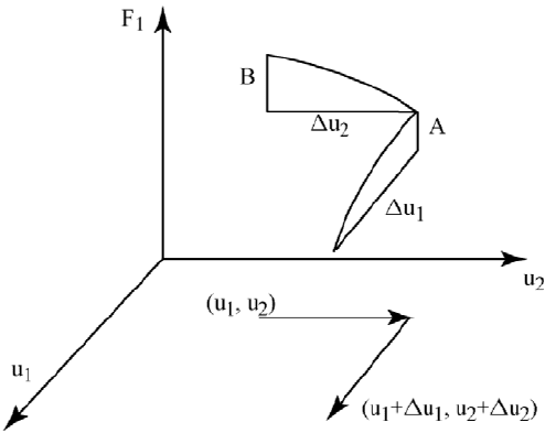
Figure 4.2.1: Change in F

straight line. Then ﬁnd the root of the equation associated with this straight

line. We make use of the approximation

i  i

({){= (4.2.4)

The equation for the straight line at iteration

p is

(

|  i({

) = i

({

)({  {

)= (4.2.5)

Deﬁne

{

p+1

so that | = 0 and solve for {

p+1

to obtain Newton’s algorithm

{

p+1

= {

 i({

)@i

({

)= (4.2.6)

The derivation of Newton’s method for more than one equation and one

unknown requires an analog of the approximation in (4.2.4). Consider

(x)

as a function of

q variables x

. If only the m component of x changes, then

(4.2.4) will hold with

{ replaced by x

and i({) replaced by I

(x). If all of the

components change, then the net change in I

(x) can be approximated by sum

of the partial derivatives of

(x) with respect to x

times the change in x

I

= I

+ x

> · · · > x

+ x

)  I

> · · · > x

)

 I

(x)x

+ · · · + I

(x)x

= (4.2.7)

For

q = 2 this is depicted by Figure 4.2.1 with l = 1 and

I

= D + E where

D  I

(x)x

and E  I

(x)x

4.2. NONLINEAR HEAT TRANSFER IN A WIRE 155

The equation approximations in (4.2.7) can be put into matrix form

I  I

(x)x (4.2.8)

where

I = [

I

· · · I

]

and x = [

x

· · · x

]

are q × 1

column vectors, and I

(x) is deﬁned as the q×q derivative or Jacobian matrix



· · · I

Newton’s method is obtained by letting x = x

> x = x

p+1

 x

and

I = 0I (x

)= The vector approximation in (4.2.8) is replaced by an equality

to get

0  I ( x

) = I

)(x

p+1

 x

)= (4.2.9)

This vector equation can be solved for

p+1

, and we have the q variable Newton

method

p+1

= x

 I

p+1

)

1

I (x

)= (4.2.10)

In practice the inverse of the Jacobian matrix is not used, but one must ﬁnd

the solution,

x, of

 I (x

) = I

)x= (4.2.11)

Consequently, Newton’s method consists of solving a sequence of linear prob-

lems. One usually stops when either

I is "small", or x is "small "

Newton Algorithm.

choose initial x

for m = 1,maxit

compute

I (x

) and I

)

solve

)x = I (x

)

p+1

= x

+ x

test for convergence

endloop.

Example 1. Let

q = 2, I

(x) = x

+ x

 1 and I

(x) = x

 x

 1@2= The

Jacobian matrix is 2×2, and it will be nonsingular if both variables are nonzero

(x) =



2x

= (4.2.12)

If the initial guess is near a solution in a particular quadrant, then Newton’s

method may converge to the solution in that quadrant.

Example 2. Consider the nonlinear di

erential equation for the radiative heat

transfer problem in (4.2.1)-(4.2.3) where

(x) = k

i(x

) + x

l1

 2x

+ x

l+1

= 0= (4.2.13)

The Jacobian matrix is easily computed and must be tridiagonal because each

(x) only depends on x

l1

, x

and x

l+1

156 CHAPTER 4. NONLINEAR AND 3D MODELS

(x) =

)  2 1

)  2

1 k

)  2

For the Stefan cooling model where the absolute temperature is positive i

(x) ?

0= Thus, the Jacobian matrix is strictly diagonally dominant and must be non-

singular so that the solve step can be done in Newton’s method.

4.2.5 Implementation

The following is a MATLAB code, which uses Newton’s metho d to solve the 1D

diusion problem with heat loss due to radiation. We have used the MATLAB

command A\d to solve each linear subproblem. One could use an iterative

method, and this might be the best way for larger problems where there is

diusion of heat in more than one direction.

In the M

ATLA B code nonlin.m the Newton iteration is done in the outer loop

in lines 13-36. The inner loop in lines 14-29 recomputes the Jacobian matrix

by rows

I S = I

(x) and updates the column vector I = I (x). The solve step

and the update to the approximate solution are done in lines 30 and 31. In

lines 32-35 the Euclidean norm of the residual is used to test for convergence.

The output is generated by lines 37-41.

MATLAB Codes nonlin.m, fnonl.m and fnonlp.m

1. clear;

2. % This code is for a nonlinear ODE.

3. % Stefan radiative heat lose is modeled.

4. % Newton’s method is used.

5. % The linear steps are solved by A\d.

6. uo = 900.;

7. n = 19;

8. h = 1./(n+1);

9. FP = zeros(n);

10. F = zeros(n,1);

11. u = ones(n,1)*uo;

12. % begin Newton iteration

13. for m =1:20

14. for i = 1:n %compute Jacobian matrix

15. if i==1

16. F(i) = fnonl(u(i))*h*h + u(i+1) - 2*u(i) + uo;

17. FP(i,i) = fnonlp(u(i))*h*h - 2;

18. FP(i,i+1) = 1;

19. elseif i

20. F(i) = fnonl(u(i))*h*h + u(i+1) - 2*u(i) + u(i-1);

4.2. NONLINEAR HEAT TRANSFER IN A WIRE 157

Table 4.2.1: Newton’s Rapid Convergence

m Norm of F

1 706.1416

2 197.4837

3 049.2847

4 008.2123

5 000.3967

6 000.0011

7 7.3703e-09

21. FP(i,i) = fnonlp(u(i))*h*h - 2;

22. FP(i,i-1) = 1;

23. FP(i,i+1) = 1;

24. else

25. F(i) = fnonl(u(i))*h*h - 2*u(i) + u(i-1) + uo;

26. FP(i,i) = fnonlp(u(i))*h*h - 2;

27. FP(i,i-1) = 1;

28. end

29. end

30. du = FP\F; % solve linear system

31. u = u - du;

32. error = norm(F);

33. if error

?.0001

34. break;

35. end

36. end

37. m;

38. error;

39. uu = [900 u’ 900];

40. x = 0:h:1;

41. plot(x,uu)

function fnonl = fnonl(u)

fnonl = .00000005*(300^4 - u^4);

function fnonlp = fnonlp(u)

fnonlp = .00000005*(-4)*u^3;

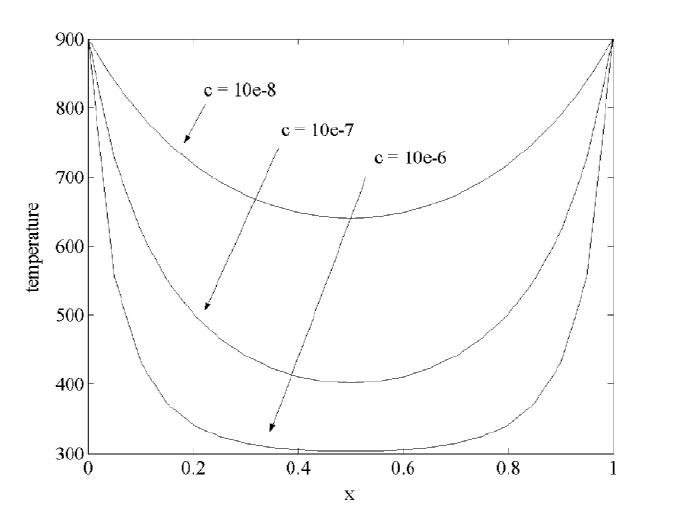
We have experimented with

f = 10

8

> 10

7

and 10

6

f the more the cooling, that is, the lower the

temperature. Recall, from (4.2.1) f = (2%@u)@N so variable %> N or u can

change

The next calculations were done to illustrate the very rapid convergence of

Newton’s method. The second column in Table 4.2.1 has norms of the residual

as a function of the Newton iterations

.The curves in Figure

4.2.2 indicate the larger the

158 CHAPTER 4. NONLINEAR AND 3D MODELS

Figure 4.2.2: Temperatures for Variable c

4.2.6 Assessment

Nonlinear problems are very common, but they are often linearized by using

linear Taylor polynomial approximations of the nonlinear terms. This is done

because it is easier to solve one linear problem than a nonlinear problem where

one must solve a sequence of linear subproblems. However, Newton’s metho d

has, under some assumption on F(u), the two very important properties of local

convergence and quadratic convergence. These two properties have contributed

to the wide use and many variations of Newton’s method for solving nonlinear

algebraic systems.

Another nonlinear method is a Picard method in which the nonlinear terms

are evaluated at the previous iteration, and the resulting linear problem is

solved for the next iterate. For example, consider the problem

x

{{

= i(x)

with

x given on the boundary. Let x

be given and solve the linear problem

x

p+1

{{

= i(x

) for the next iterate x

p+1

. This method does not always

converge, and in general it does not converge quadratically.

4.2.7 Exercises

1. Apply Newton’s method to example 1 with q = 2. Experiment with

dierent initial guesses in each quadrant. Observe local and quadratic conver-

gence.

2. Apply Newton’s method to the radiative heat transfer problem. Exper-

iment with di

erent q> hsv> O and emissivities. Observe local and quadratic