White R.E. Computational Mathematics: Models, Methods, and Analysis with MATLAB and MPI
Подождите немного. Документ загружается.

3.3. FLUID FLOW IN A 2D POROUS MEDIUM 119
MATLAB Code por2d.m
1. % Steady state saturated 2D porous flow.
2. % SOR is used to solve the algebraic system.
3. % SOR parameters
4. clear;
5. maxm = 500;
6. eps = .01;
7. ww = 1.97;
8. % Porous medium data
9. nx = 50;
10. ny = 20;
11. cond = 10.;
12. iw = 15;
13. jw = 12;
14. iwp = 32;
15. jwp = 5;
16. R_well = -250.;
17. uleft = 100. ;
18. uright = 100.;
19. for j=1:ny+1
20. u(1,j) = uleft;
21. u(nx+1,j) = uright;
22. end
23. for j =1:ny+1
24. for i = 2:nx
25. u(i,j) = 100.;
26. end
27. end
28. W = 1000.;
29. L = 5000.;
30. dx = L/nx;
31. rdx = 1./dx;
32. rdx2 = cond/(dx*dx);
33. dy = W/ny;
34. rdy = 1./dy;
35. rdy2 = cond/(dy*dy);
36. % Calibrate R_well to be independent of the mesh
37. R_well = R_well/(dx*dy);
38. xw = (iw)*dx;
39. yw = (jw)*dy;
40. for i = 1:nx+1
41. x(i) = dx*(i-1);
42. end
43. for j = 1:ny+1
© 2004 by Chapman & Hall/CRC
120 CHAPTER 3. POISSON EQUATION MODELS
44. y(j) = dy*(j-1);
45. end
46. % Execute SOR Algorithm
47. nunkno = (nx-1)*(ny+1);
48. m = 1;
49. numi = 0;
50. while ((numi
?nunkno)*(m?maxm))
51. numi = 0;
52. % Interior nodes
53. for j = 2:ny
54. for i=2:nx
55. utemp = rdx2*(u(i+1,j)+u(i-1,j));
56. utempp = utemp + rdy2*(u(i,j+1)+u(i,j-1));
57. utemp = utempp/(2.*rdx2 + 2.*rdy2);
58. if ((i==iw)*(j==jw))
59. utemp=(utempp+R_well)/(2.*rdx2+2.*rdy2);
60. end
61. if ((i==iwp)*(j==jwp))
62. utemp =(utempp+R_well)/(2.*rdx2+2.*rdy2);
63. end
64. utemp = (1.-ww)*u(i,j) + ww*utemp;
65. error = abs(utemp - u(i,j)) ;
66. u(i,j) = utemp;
67. if (error
?eps)
68. numi = numi +1;
69. end
70. end
71. end
72. % Bottom nodes
73. j = 1;
74. for i=2:nx
75. utemp = rdx2*(u(i+1,j)+u(i-1,j));
76. utemp = utemp + 2.*rdy2*(u(i,j+1));
77. utemp = utemp/(2.*rdx2 + 2.*rdy2 );
78. utemp = (1.-ww)*u(i,j) + ww*utemp;
79. error = abs(utemp - u(i,j)) ;
80. u(i,j) = utemp;
81. if (error
?eps)
82. numi = numi +1;
83. end
84. end
85. % Top nodes
86. j = ny+1;
87. for i=2:nx
88. utemp = rdx2*(u(i+1,j)+u(i-1,j));
© 2004 by Chapman & Hall/CRC
3.3. FLUID FLOW IN A 2D POROUS MEDIUM 121
89. utemp = utemp + 2.*rdy2*(u(i,j-1));
90. utemp = utemp/(2.*rdx2 + 2.*rdy2);
91. utemp = (1.-ww)*u(i,j) + ww*utemp;
92. error = abs(utemp - u(i,j));
93. u(i,j) = utemp;
94. if (error
?eps)
95. numi = numi +1;
96. end
97. end
98. m = m+1;
99. end
100. % Output to Terminal
101. m
102. ww
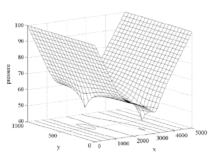
103. meshc(x,y,u’)
the pressure drops from 100 to around 45. This required 199 SOR iterations,
and SOR parameter
z = 1=97 was found by numerical experimentation. This
numerical approximation may have significant errors due either to the SOR
convergence criteria hsv = =01 in line 6 being too large or to the mesh size
in lines 9 and 10 being too large. If
hsv = =001, then 270 SOR iterations are
required and the solution did not change by much. If hsv = =001, q| is doubled
from 20 to 40, and the
mz and mzs are also d oubled so that the wells are located
in the same position in space, then 321 SOR iterations are computed and little
di
erence in the graphs is noted. If the flow rate at both wells is increased from
250. to 500., then the pressure should drop. Convergence was attained in 346
SOR iterations for hsv = =001, q{ = 50 and q| = 40, and the graph s hows the
pressure at the second well to be negative, which indicates the well has gone
dry!
3.3.6 Assessment
This porous flow model has enough assumptions to rule out many real applica-
tions. For groundwater problems the soils are usually not fully saturated, and
the hydraulic conductivity can be highly nonlinear or vary with s pace according
to the soil types. Often the soils are very heterogeneous, and the soil properties
are unknown. Porous flows may require 3D calculations and irregularly shaped
domains. The good news is that the more complicated models have many sub-
problems, which are similar to our present models from heat di
usion and fluid
flow in saturated porous media.
3.3.7 Exercises
1. Consider the groundwater problem. Experiment with the choice of z and
hsv. Observe the number of iterations required for convergence.
© 2004 by Chapman & Hall/CRC
The graphical output is given in Figure 3.3.3 where there are two wells and
122 CHAPTER 3. POISSON EQUATION MODELS
Figure 3.3.3: Pressure for Two Wells
2. Experiment with the mesh sizes
q{ and q|, and convince yourself the
discrete problem has converged to the continuous problem.
3. Consider the groundwater problem. Experiment with the physical para-
meters
N = frqg, Z , O and pump rate U = U_zhoo.
4. Consider the groundwater problem. Experiment with the number and
location of the wells.
3.4 Ideal Fluid Flow
3.4.1 Introduction
An ideal fluid is a steady state flow in 2D that is incompressible and has no
circulation. In this case the velo city of the fluid can be represented by a stream
function, which is a solution of a partial di
erential equation that is similar to
the 2D heat di
usion and 2D porous flow models. The applied problem could
be viewed as a first model for flow of a shallow river about an object, and
the numerical solution will also be given by a variation of the previous SOR
M
ATLAB codes.
3.4.2 Applied Area
Because the fluid is not com-
pressible, it must significantly increase its speed in order to pass near the ob-
stacle. This can cause severe erosion of the nearby soil. The problem is to
© 2004 by Chapman & Hall/CRC
Figure 3.4.1 depicts the flow about an obstacle.
3.4. IDEAL FLUID FLOW 123
Figure 3.4.1: Ideal Flow About an Obstacle
determine these velocities of the fluid given the upstream velocity and the lo-
cation and shape of the obstacle.
3.4.3 Model
We assume the velocity is a 2D steady state incompressible fluid flow. The
incompressibility of the fluid can be characterized by the divergence of the
velocity
x
{
+ y
|
= 0= (3.4.1)
The circulation or rotation of a fluid can be described by the curl of the velocity
vector. In 2D the curl of (u, v) is
y
{
x
|
. Also the discrete form of this gives
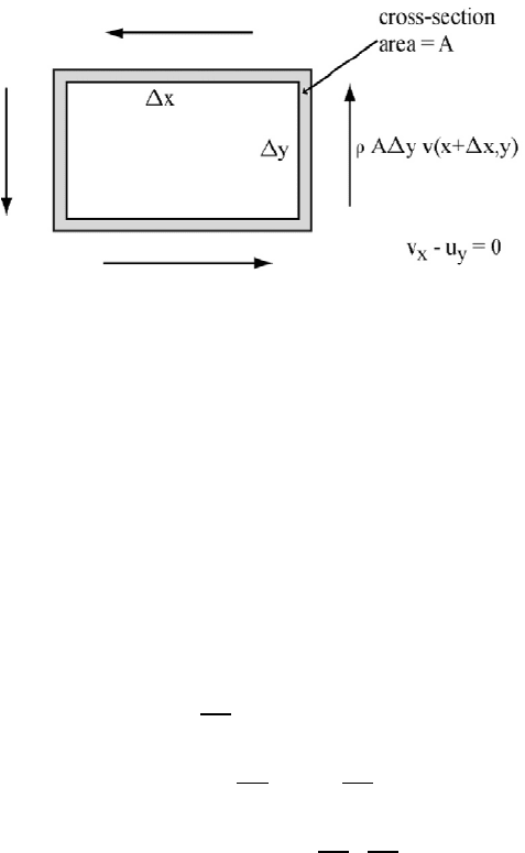
some insight to its meaning. Consider the loop about the rectangular region
Let A be the cross-sectional area in this loop. The
momentum of the vertical segment of the right side is
D| y({ + {> |). The
circulation or angular momentum of the loop about the tube with cross-section
area D and density is
D|(y({ + {> |) y({> |)) D{(x({> | + |) x({> |))=
Divide by (D|{) and let { and | go to zero to get y
{
x
|
= If there is
no circulation, then this must be zero. The fluid is called irrotational if
y
{
x
|
= 0= (3.4.2)
An ideal 2D steady state fluid flow is defined to be incompressible and
irrotational so that both equations (3.4.1) and (3.4.2) hold. One can use the
incompressibility condition and Green’s theorem (more on this later) to show
that there is a stream function,
, such that
(
{
>
|
) = (y> x)= (3.4.3)
The irrotational condition and (3.4.3) give
y
{
x
|
= (
{
)
{
(
|
)
|
= 0=
© 2004 by Chapman & Hall/CRC
given in Figure 3.4.2.
124 CHAPTER 3. POISSON EQUATION MODELS
Figure 3.4.2: Irrotational 2D Flow y
{
x
|
= 0
x
0
> 0), then let = x
0
|=
If the velocity at the right in Figure is (x> 0), then let
{
= 0= Equation (3.4.4)
and these boundary conditions give the ideal fluid flow model.
We call
a stream function because the curves ({()> |()) defined by
setting to a constant are parallel to the velocity vectors (x> y). In order
to see this, let
({()> |()) = f, compute the derivative with respect to and
use the chain rule
0 =
g
g
({()> |())
=
{
g{
g
+
|
g|
g
= (y> x) · (
g{
g
>
g|
g
)=
Since (x> y) · (y> x) = 0> (x> y) and the tangent vector to the curve given by
({()> |()) = f must be parallel.
Ideal Flow Around an Obstacle Model.
{{
||
= 0 for ({> |) 5 (0> O) × (0> Z )>
= x
0
| for { = 0 (x = x
0
)>
= x
0
Z for | = Z (y = 0)
= 0 for | = 0 or ({> |) on the obstacle and
{
= 0 for { = O (y = 0)=
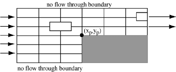
3.4.4 Method
Use the finite dierence method coupled with the SOR iterative scheme. For
the (
{|) cells in the interior this is similar to the 2D heat diusion problem.
For the portions of the boundary where a derivative is set equal to zero on a half
cell (
{@2 |) as in Figure 3.4.1, insert some additional code inside the SOR
loop. In the obstacle model where
{
= 0 at { = O we have half cells ({@2
© 2004 by Chapman & Hall/CRC
If the velocityupstream to the left in Figure 3.4.1 is (
3.4. IDEAL FLUID FLOW 125
|). The finite dierence equation in equation (3.4.5) and corresponding line
in (3.4.6) of SOR code with
x = > g{ = { and g| = | are
0 =
[(0)@g{ (x(l> m) x(l 1> m))@g{]@g{@2
[(x(l> m + 1) x(l> m))@g|
(x(l> m) x(l> m 1))@g|]@g| (3.4.4)
xwhps = (2 x(l 1> m)@(g{ g{) +
(
x(l> m + 1) + x(l> m 1))@(g| g|))
@(2@(g{ g{) + 2@(g| g|))
x(l> m) = (1 z) x(l> m) + z xwhps= (3.4.5)
3.4.5 Implementation
The MATLAB code ideal2d.m has a similar structure as por2d.m, and also
it uses the SOR scheme to approximate the solution to the algebraic system
associated with the ideal flow about an obstacle. The obstacle is given by
indices of the point (
ls> ms) as is done in lines 11,12. Other input data is
given in lines 4-39. The SOR scheme is executed using the while loop in lines
46-90. The SOR calculations for the various nodes are done in three groups:
the interior bottom nodes in lines 48-62, the interior top nodes in lines 62-75
and the right boundary nodes in lines 76-88. Once the SOR iterations have
been completed, the output in lines 92-94 prints the number of SOR iterations,
the SOR parameter and the contour graph of the stream line function via the
M
ATLA B command contour(x,y,u’).
MATLAB Code ideal2d.m
1. % This code models flow around an obstacle.
2. % SOR iterations are used to solve the system.
3. % SOR parameters
4. clear;
5. maxm = 1000;
6. eps = .01;
7. ww = 1.6;
8. % Flow data
9. nx = 50;
10. ny = 20;
11. ip = 40;
12. jp = 14;
13. W = 100.;
14. L = 500.;
15. dx = L/nx;
16. rdx = 1./dx;
© 2004 by Chapman & Hall/CRC
adarkened rectangle in Figure 3.4.1, and can be identified by indicating the
126 CHAPTER 3. POISSON EQUATION MODELS
17. rdx2 = 1./(dx*dx);
18. dy = W/ny;
19. rdy = 1./dy;
20. rdy2 = 1./(dy*dy);
21. % Define Boundary Conditions
22. uo = 1.;
23. for j=1:ny+1
24. u(1,j) = uo*(j-1)*dy;
25. end
26. for i = 2:nx+1
27. u(i,ny+1) = uo*W;
28. end
29. for j =1:ny
30. for i = 2:nx+1
31. u(i,j) = 0.;
32. end
33. end
34. for i = 1:nx+1
35. x(i) = dx*(i-1);
36. end
37. for j = 1:ny+1
38. y(j) = dy*(j-1);
39. end
40. %
41. % Execute SOR Algorithm
42. %
43. unkno = (nx)*(ny-1) - (jp-1)*(nx+2-ip);
44. m = 1;
45. numi = 0;
46. while ((numi
?unkno)*(m?maxm))
47. numi = 0;
48. % Interior Bottom Nodes
49. for j = 2:jp
50. for i=2:ip-1
51. utemp = rdx2*(u(i+1,j)+u(i-1,j));
52. utemp = utemp + rdy2*(u(i,j+1)+u(i,j-1));
53. utemp = utemp/(2.*rdx2 + 2.*rdy2);
54. utemp = (1.-ww)*u(i,j) + ww*utemp;
55. error = abs(utemp - u(i,j));
56. u(i,j) = utemp;
57. if (error
?eps)
58. numi = numi +1;
59. end
60. end
61. end
© 2004 by Chapman & Hall/CRC
3.4. IDEAL FLUID FLOW 127
62. % Interior Top Nodes
63. for j = jp+1:ny
64. for i=2:nx
65. utemp = rdx2*(u(i+1,j)+u(i-1,j));
66. utemp = utemp + rdy2*(u(i,j+1)+u(i,j-1));
67. utemp = utemp/(2.*rdx2 + 2.*rdy2);
68. utemp = (1.-ww)*u(i,j) + ww*utemp;
69. error = abs(utemp - u(i,j)) ;
70. u(i,j) = utemp;
71. if (error
?eps)
72. numi = numi +1;
73. end
74. end
75. end
76. % Right Boundary Nodes
77. i = nx+1;
78. for j = jp+1:ny
79. utemp = 2*rdx2*u(i-1,j);
80. utemp = utemp + rdy2*(u(i,j+1)+u(i,j-1));
81. utemp = utemp/(2.*rdx2 + 2.*rdy2);
82. utemp = (1.-ww)*u(i,j) + ww*utemp;
83. error = abs(utemp - u(i,j));
84. u(i,j) = utemp;
85. if (error
?eps)
86. numi = numi +1;
87. end
88. end
89. m = m +1;
90. end
91. % Output to Terminal
92. m
93. ww
94. contour(x,y,u’)
The obstacle model uses the parameters
O = 500> Z = 100 and x
0
= 1.
Since
x
0
= 1, the stream function must equal 1| in the upstream position, the
{ component of the velocity is x
0
= 1, and the |
component of the velocity will be zero. The graphical output gives the contour
lines of the stream function. Since these curves are much closer near the exit,
the right side of the figure, the
{ component of the velocity must be larger
above the obstacle. If the obstacle is made smaller, then the exiting velocity
will not be as large.
© 2004 by Chapman & Hall/CRC
left side of Figure 3.4.1. The
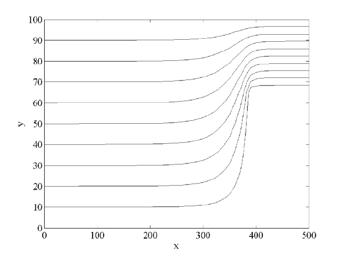
128 CHAPTER 3. POISSON EQUATION MODELS
Figure 3.4.3: Flow Around an Obstacle
3.4.6 Assessment
This ideal fluid flow model also has enough assumptions to rule out many real
applications. Often there is circulation in flow of water, and therefore, the
irrotational assumption is only true for slow moving fluids in which circulation
does not develop. Air is a compressible fluid. Fluid flows may require 3D
calculations and irregularly shaped domains. Fortunately, the more complicated
models have many subproblems which are similar to our present models from
heat di
usion, fluid flow in saturated porous medium and ideal fluid flow.
The existence of stream functions such that (
{
>
|
) = (y> x) needs t o
be established. Recall the conclusion of Green’s Theorem where
is a simply
connected region in 2D with boundary
F given by functions with piecewise
continuous first derivatives
I
F
S g{ + Tg| =
ZZ
T
{
S
|
g{g|= (3.4.6)
Suppose
x
{
+y
|
= 0 and let T = x and S = y. Since T
{
S
|
= (x)
{
(y)
|
=
0
> then the line integral about a closed curve will always be zero. This means
that the line integral will be independent of the path taken between two points.
Define the stream function to be the line integral of (
S> T) = (y> x) starting
at some (
{
0
> |
0
) and ending at ({> |). This is single valued because the line
integral is independent of the p ath taken. In order to show (
{
>
|
) = (y> x),
© 2004 by Chapman & Hall/CRC