Warren J., Weimer H. Subdivision Methods for Geometric Design. A Constructive Approach

Подождите немного. Документ загружается.

264 CHAPTER 8 Spectral Analysis at an Extraordinary Vertex

Note that we have not assumed an explicit subdivision rule at the extraordinary

vertex

v. Instead, we have written this rule so as to weight the vertex v by weight

1 − w[n] and the neighbors of v by weights

w[n]

Deleting the uppermost row and leftmost column of

S yields a (3 × 3) block

circulant submatrix

), where 0 ≤ i < 3 and 0 ≤ j < 3. To compute the eigenvalues

and eigenvectors of

S, we first compute the eigenvalues and eigenvectors of

)

and then extend these vectors to form eigenvectors of S. The eigenvalues and

eigenvectors of

) can be computed by examining the spectral structure of the

matrix

[x]):

⎛

⎜

⎝

x +

−1

x +

−1

⎞

⎟

⎠

. (8.14)

This lower triangular matrix has three eigenvalues that correspond to the entries

on its diagonal:

x +

−1

, and

. Evaluating these three eigenvalues at

x = ω

for 0 ≤ h < n yields the corresponding 3n eigenvalues of (C

). For example,

n == 4, the four eigenvalues of (C

) associated with

x +

−1

are

and

. The remaining eight eigenvalues of (C

) consist of four copies of

and four

copies of

Note that the

n-fold symmetry of the mesh M used in defining S gave rise to

the block circulant structure of

). This symmetry also manifests itself during

the construction of the eigenvectors of

). In particular, the eigenvectors of the

matrix

[x]) correspond to the restriction of the eigenvectors of (C

) to a sin-

gle sector of the underlying mesh

M. The multiplication of the components of

these eigenvectors of

[x]) by powers of x where x

== 1 corresponds to rotating

the components of this eigenvector in the complex plane to form the associated

eigenvector of

) defined over all n sectors of M.

The matrix

[x]) of equation 8.14 has three eigenvectors of the form

{1,

1+x

1+13x+x

2+5x +2x

}, {0, x, 1 + x}, and {0, 0, 1}. The corresponding 3n eigenvectors of

) are as shown in equation 8.13, with x being evaluated at ω

for 0 ≤ h < n.For

example, if

n == 4, the four eigenvectors of (C

) corresponding to {0, x, 1 + x} have

the form

{0, 0, 0, 0, x, x

, x

,(1 + x), (1 + x)x,(1 + x)x

,(1 + x)x

8.3 Verifying the Smoothness Conditions for a Given Scheme 265

where x = i

for 0 ≤ h < 4. The remaining eight eigenvectors of (C

) corresponding

1+x

1+13x+x

2+5x +2x

and

{0, 0, 1} are constructed in a similar manner.

Given these eigenvectors for

), we next form potential eigenvectors for the

subdivision matrix

S by prepending an initial zero to these vectors. For the 3n − 3

eigenvectors (C

) corresponding to x taken at ω

where 0 < h < n, these extended

vectors have the property that they also annihilate the uppermost row of

S. There-

fore, these extended vectors are eigenvectors of

S whose associated eigenvalues are

simply the corresponding eigenvalues of

). Most importantly, the eigenvalue

x +

−1

of (c

[x]) gives rise to n − 1 eigenvalues of S of the form

−h

Cos



2πh



for

0 < h < n. Note that these eigenvalues lie in the range (

) and reach a

maximum at

h = 1, n − 1. In particular, we let λ[n] denote this maximal double

eigenvalue of

; that is,

λ[n] =

Cos



2π



For appropriate choices of w[n], this double eigenvalue λ[n] is the subdominant

eigenvalue of the subdivision matrix

S. Observe that the associated eigenvectors

used in defining the characteristic map are independent of the weight function

w[n]. (In the next section, we will show that the characteristic map defined by

these eigenvectors is regular.)

The remaining four of the

3n + 1 eigenvectors of S have entries that are con-

stant over each block of

S. The four eigenvalues associated with these eigenvectors

are eigenvalues of the

4 × 4 matrix formed by summing any row of each block in

the matrix

S; that is,

⎛

⎜

⎝

1 − w[n] w[n] 0 0

⎞

⎟

⎠

(Note that the 3 × 3 submatrix on the lower right is simply (c

[1]).)

Because the eigenvalues of this matrix are

− w[n],

, the full spectrum

of the local subdivision matrix

S (and its infinite counterpart S) has the form

266 CHAPTER 8 Spectral Analysis at an Extraordinary Vertex

1, λ[n], λ[n],

− w[n] with all of the remaining eigenvalues having an absolute value

less than

λ[n] ( ). Our goal is to choose the weight function w[n] such that λ[n] >

− w[n]|. To this end, we substitute the definition of λ[n] into this expression and

observe that this inequality simplifies to

1 − Cos

2π

< w[n] <

4 + Cos

2π

(8.15)

Any choice for w[n] that satisfies this condition yields a subdivision matrix S whose

spectrum has the form

1 >λ[n] == λ[n] > |

−w[n]|

. Therefore, by Theorem 8.4, the

limit functions associated with such a scheme are smooth at extraordinary vertices.

For example, linear subdivision plus averaging (see section 7.3.1) causes the weight

function

w[n] to be the constant

. This choice for w[n] satisfies equation 8.15 for

all

n > 3, and consequently linear subdivision plus averaging converges to smooth

limit functions at extraordinary vertices with valences greater than three. However,

for

n == 3, the subdivision matrix S has the spectrum 1,

, ..., and, as observed

previously, the resulting scheme is continuous, but not smooth, at the extraordinary

vertices of this valence. (An alternative choice for

w[n] that satisfies equation 8.15

for all valences and reproduces the uniform weight

w[6] ==

is w[n] =

n+2

Loop’s subdivision rule uses a subtler choice for

w[n]. In particular, Loop sets

the weight function

w[n] to have the value

− λ[n]

. This choice satisfies equation

8.15 for all

n ≥ 3 and yields a subdivision matrix S whose spectrum has the form

1, λ[n], λ[n], ..., λ[n]

, .... This particular choice for w[n] is motivated by an attempt

to define a subdivision rule that is

continuous at extraordinary vertices. Unfor-

tunately, the eigenfunction associated with the eigenvalue

λ[n]

does not reproduce

a quadratic function as required by Theorem 8.5, and therefore cannot be

at the

extraordinary vertex

However, this associated eigenfunction does have the property that its curva-

ture is bounded (but discontinuous) at

v (see Peters and Umlauf [118] for details).

For valences

3 ≤ n ≤ 6, the spectrum of S has the form 1, λ[n], λ[n], λ[n]

, ... (i.e.,

there are no other eigenvalues between

λ[n] and λ[n]

). Therefore, due to Theo-

rem 8.4, Loop’s scheme produces limit surfaces with bounded curvature for these

valences. This bound on the curvature is particularly important in some types of

milling applications. In a similar piece of work, Reif and Schr

oder [130] show that

the curvature of a Loop surface is square integrable, and therefore Loop surfaces

can be used in a finite element method for modeling the solution to thin shell

equations [22].

8.3 Verifying the Smoothness Conditions for a Given Scheme 267

An almost identical analysis can be used to derive the spectral structure for

Catmull-Clark subdivision (and its quadrilateral variants). The crux of the analysis

is deriving an analog to the

3 × 3 matrix of equation 8.14. For quad meshes, there

are

6n vertices in the two-ring of the vertex v (excluding v). If we order the indices

ij of the six vertices in a single quadrant as 10, 11, 20, 12, 21, and 22, the appropriate

6 × 6 matrix is

⎛

⎜

⎝

x +

−1

0000

x +

−1

⎞

⎟

⎠

Computing the eigenvalues and eigenvectors of this matrix and evaluating them

x = ω

for 0 ≤ h < n leads to the desired spectral decomposition of S. Reif and

Peters [116] perform such an analysis in full detail and show that Catmull-Clark

subdivision produces

limit functions at extraordinary vertices of all valences.

8.3.3 Proving Regularity of the Characteristic Map

To complete our proof that Loop’s scheme produces smooth limit surfaces, we

must verify that the characteristic map for this scheme is regular at an extraordinary

vertex of arbitrary valence. In this section, we outline a proof of regularity for the

characteristic map arising from Loop’s scheme. The basic approach is to compute

the pair of eigenvectors corresponding to the double eigenvalue

λ[n] and show

that the Jacobian of the resulting characteristic map

ψ[h, x, y] has the same sign

everywhere; that is,

Det



(1,0)

[h, x, y] ψ

(0,1)

[h, x, y]

(1,0)

[h, x, y] ψ

(0,1)

[h, x, y]



= 0

(8.16)

for all x, y ≥ 0, where ψ ={ψ

, ψ

}. This condition on the Jacobian of ψ prevents

ψ from folding back on itself locally and is sufficient to guarantee that the map is

regular (see Fleming [63] for more details). In practice, we orient the meshes used

268 CHAPTER 8 Spectral Analysis at an Extraordinary Vertex

in computing this Jacobian such that the resulting determinant is strictly positive

for regular characteristic maps.

As observed in the previous section, the range on which this condition must

be verified can be reduced significantly via equation 8.8. Because

λ[n] is real and

positive, applying the affine transformation

λ[n] 0

0 λ[n]

to the map

ψ does not affect

its regularity. Thus, if we can prove that

ψ satisfies equation 8.16 on an annulus

surrounding

v of sufficient width, the recurrence of equation 8.8 implies that ψ sat-

isfies equation 8.16 everywhere except at

v. Because the subdominant eigenvectors

used in defining the characteristic map arise from the principal

nth root of unity

, this annulus winds around v exactly once, and the corresponding characteristic

map

ψ is also regular at the origin.

For surface schemes supported on the two-ring, this annulus typically consists

of those faces that lie in the two-ring but not in the one-ring of

v. The advantage

of this choice is that the behavior of the scheme on this annulus is determined

entirely by the uniform subdivision rules used in

S. For triangular schemes, such

as Loop’s scheme, this annulus consists of the region

1 ≤ x + y ≤ 2 composed of

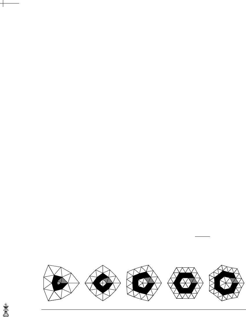
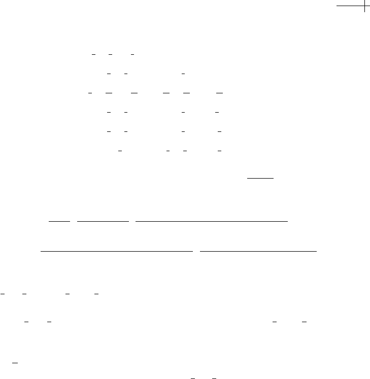
triangular faces with 3 triangles per wedge (see Figure 8.7). In this section, we

sketch a computational proof that the characteristic map

ψ for Loop’s scheme (and

its triangular variants) is regular. This method is very similar to an independently

derived method given in Zorin et al. [171]. Variants of either the current method

or Zorin’s method can be used to prove that the characteristic map for quadrilateral

schemes is also regular.

Our first task in this proof is to compute the two eigenvectors used in defining

the characteristic map, that is, the eigenvectors associated with the double eigen-

value

λ[n]. In particular, we need the entries of these eigenvectors over the three-

ring of the extraordinary vertex

v because this ring determines the behavior of the

characteristic map on the two-ring of

v (i.e., the annulus 1 ≤ x + y ≤ 2). Recall that

this double eigenvalue arose from evaluating the eigenvalue

1+3x +x

of the matrix

[x]) of equation 8.14 at x = ω

and x = ω

−1

. Extending the matrix (c

[x]) to the

Figure 8.7 The annulus used in verifying regularity of the characteristic map for Loop’s scheme.

8.3 Verifying the Smoothness Conditions for a Given Scheme 269

three-ring of v yields a new matrix of the form

⎛

⎜

⎝

x +

−1

0 0 000

0 000

x +

−1

000

x000

000

−1

000

⎞

⎟

⎠

Now, the eigenvector associated with the eigenvalue

1+3x +x

for this extended

matrix is the vector



1 + x

1 + 13x + x

2 + 5x + 2x

x(2 + 32x + 87x

+ 55x

+ 7x

)

(1 + x)(2 + 11x + 19x

+ 11x

+ 2x

)

x(7 + 55x + 87x

+ 32x

+ 2x

)

(1 + x)(2 + 11x + 19x

+ 11x

+ 2x

)

3x(5 + 23x + 5x

)

2 + 11x + 19x

+ 11x

+ 2x

Evaluating this eigenvector at x = ω

yields a complex eigenvector of the form

+iz

, where z

and z

are the real eigenvectors associated with the double eigen-

value

λ[n]. (Evaluating at x = ω

−1

yields a complex conjugate eigenvector of the

form

− iz

.) As observed previously, these real eigenvectors z

and z

define the

behavior of the characteristic map on a single sector of

M. To construct the char-

acteristic map for all

n sectors, these eigenvectors can be extended to eigenvectors

S by multiplying by powers of x

for 0 < h < n. Because x

== 1, the action of

this multiplication is to rotate the entries of

+iz

in the complex plane and make

n copies of a single sector. Figure 8.7 shows a plot of the mesh resulting from this

rotation for valences ranging from

3 to 7.

To prove regularity of the corresponding characteristic maps

ψ, we must show

that

ψ satisfies the Jacobian condition of equation 8.16 on the darkened annulus of

Figure 8.7 corresponding to

1 ≤ x + y ≤ 2 for 0 ≤ h < n. Given the n-fold rotational

symmetry of

ψ, we can restrict our regularity analysis to the two gray triangles in

this annulus of Figure 8.7. The behavior of

ψ on these two triangles is determined

completely by the

4×4 submesh containing this pair of triangles. Figure 8.8 depicts

these submeshes for extraordinary vertices of valences

3 ≤ n ≤ 7.

Our final task is to show that the Jacobian condition of equation 8.16 holds over

the gray regions in question. Due to the tensor product structure of these

4 ×4 sub-

meshes, this verification can be done quite easily. Because the uniform subdivision

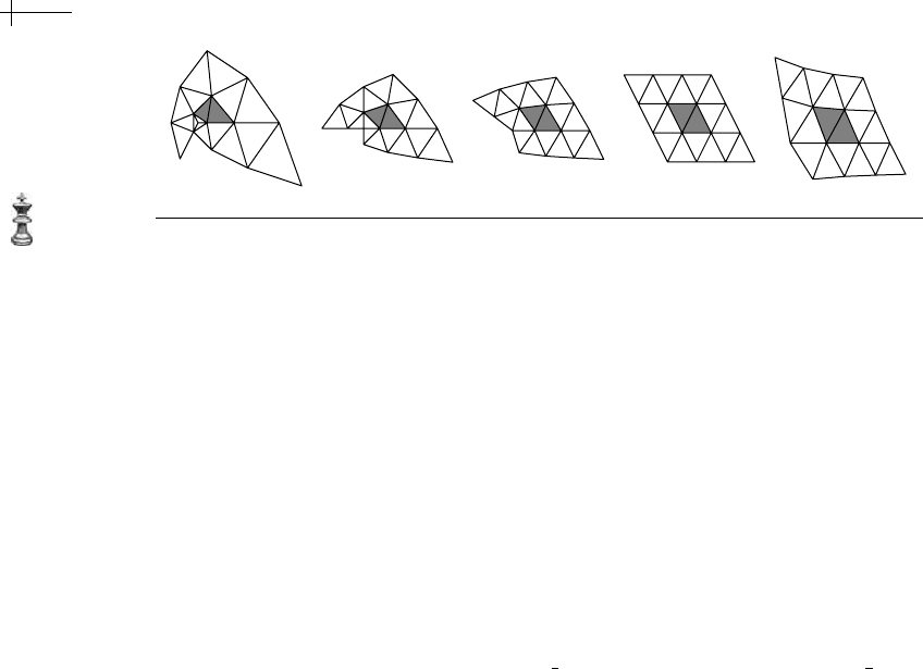
270 CHAPTER 8 Spectral Analysis at an Extraordinary Vertex

Figure 8.8 4 × 4 submeshes used in verifying regularity.

rules for our triangular schemes are based on box splines, we can compute the

directional derivatives of

ψ (i.e. ψ

(1,0)

and ψ

(0,1)

) and represent these derivatives as

box splines of lower order. The coefficients of these derivative schemes are formed

by computing directional differences between adjacent control points with respect

to the two coordinate directions. Because the basis functions associated with the

directional derivative are non-negative, the maximum and minimum values of the

four entries in the Jacobian matrix can be bounded using the convex hull property.

Representing these bounds as an interval, we can have Mathematica compute the

determinant of this matrix of intervals.

As a univariate example, consider the problem of proving regularity for the

nonuniform curve scheme of our running example. The eigenvector

associated

with the subdominant eigenvalue

had the form {..., −3, −2, −1,

, 2, 4,

6, ...}

.Ifψ[h, x] is the characteristic map for this scheme (i.e., the limit function

associated with this eigenvector

), we must show that the Jacobian of ψ[h, x],

(1)

[h, x] has the same sign for all x ≥ 0 where h = 0, 1. By applying equation 8.8,

this condition can be reduced to showing that

(1)

[h, x] has the same sign for

2 ≤ x < 4 where h = 0, 1. (Note that we use the annulus [2, 4] in place of [1, 2]

because the subdivision rules for the curve scheme are uniform over this larger

interval.) The subvectors

{−5, −4, −3, −2, −1} and {2, 4, 6, 8, 10} of z

determine the

behavior of

ψ[h, x] on the intervals [2, 4] where h = 0, 1. To bound ψ

(1)

[x] on these

intervals, we observe that the differences of consecutive coefficients in these sub-

vectors are the coefficients of the uniform quadratic B-spline corresponding to

(1)

[h, x].Forh == 0, these differences are all −1, and therefore ψ

(1)

[0, x] == − 1 for

2 ≤ x < 4. Likewise, for h == 1, the maximum and minimum of these differences

are

2, and therefore ψ

(1)

[1, x] == 2 for 2 ≤ x < 4. Thus, ψ[h, x] is regular for our curve

example.

In the bivariate case, we store the

4 × 4 submesh in a positive orientation and

compute an interval that bounds the value of the Jacobian using this method. If

this interval is strictly positive, the Jacobian is positive over the entire gray region.

8.3 Verifying the Smoothness Conditions for a Given Scheme 271

If the interval is strictly negative, the Jacobian test fails. If the interval contains zero,

the gray region is recursively subdivided into four subregions using the subdivision

rules associated with the schemes. The test is then applied to each subregion, with

failure on any subregion implying violation of the Jacobian condition.

The associated implementation contains the Mathematica functions that im-

plement this test (

). The first function, jacobian, returns an interval bound on the

value of the Jacobian for a given

4×4 mesh. The second function, regular, recursively

applies

jacobian using the uniform subdivision rule associated with the scheme. The

user can test whether the characteristic map

ψ satisfies regular for any valence n.

Ultimately, we would like to conclude that

ψ is regular for all valences n ≥3.

One solution would be to take the limit of the

4 ×4 mesh associated with our gray

region as

n →∞and then show that this limiting mesh satisfies the Jacobian con-

dition. Unfortunately, the entries in the second eigenvector

(i.e., the imaginary

part of the complex eigenvector

z) converge to zero as n →∞. The effect on the

associated

4 × 4 mesh is to compress this mesh toward the s axis. The solution to

this problem is to scale the

t component of the characteristic map by a factor of

Sin[

2π

]

(i.e., divide z

by Sin[

2π

]). This division does not affect the regularity of the

map

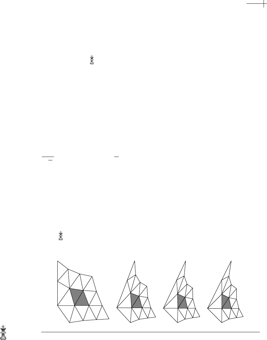
ψ and stretches the mesh in such a way that a unique limit mesh does exist as

n →∞. Figure 8.9 shows this normalized mesh for n = 8, 16, 32, ∞.

Now, we can complete our proof of regularity by explicitly testing regularity

for valences

3 ≤ n ≤ 31. Then, using Mathematica, we can compute this normalized

4 × 4 mesh as a symbolic function of n. Finally, we can verify that all character-

istic maps for valence

n ≥ 32 are regular by calling the function regular on this

symbolic normalized mesh with

n == Interval [{32, ∞}]. The associated implemen-

tation performs these calculations and confirms that

ψ is regular for all valences

n ≥ 3 ( ).

Figure 8.9 Nonuniform scaling to obtain a convergent submesh as n →∞.

272 CHAPTER 8 Spectral Analysis at an Extraordinary Vertex

8.4 Future Trends in Subdivision

This book has covered only the basics of subdivision. One of the exciting aspects

of subdivision is that it is an area in which research is actively taking place. In this

brief conclusion, we outline some of these research areas.

8.4.1 Solving Systems of Physical Equations

Chapters 4, 5, and 6 developed subdivision schemes that converge to the solutions

of a range of physical problems. The basic approach in these chapters was to con-

struct subdivision schemes that simulated the behavior of either a multilevel finite

difference solver or a multilevel finite element solver. As the authors have shown in

[162] and [163], these schemes are essentially a special type of multigrid method in

which the prediction operator has been customized to the particular physical prob-

lem. For graphical applications, this predictor is accurate enough that the smoothing

and coarse grid correction steps of traditional multigrid can be skipped. In this vein,

one area that is ripe for further research is the connection between subdivision and

multigrid. For example, techniques from traditional multigrid might lead to new,

interesting types of subdivision schemes. Conversely, techniques from subdivision

might lead to advances in multigrid solvers.

Another interesting possibility is the construction of finite element schemes

whose associated bases are defined solely through subdivision. Chapter 6 includes

two nonuniform examples of this approach: one for natural cubic splines and one

for bounded harmonic splines. Although both of these examples are functional, a

more interesting possibility is applying this idea to shapes defined as parametric

meshes. Following this approach, the solution to the associated physical problem

would be represented as an extra coordinate attached to the mesh. The advantage

of this method is that it unifies the geometric representation of a shape and its

finite element representation.

8.4.2 Adaptive Subdivision Schemes

Another area of subdivision that is ripe with promise is that of adaptive subdivision.

For univariate spline schemes, the most powerful type of adaptive subdivision in-

volves knot insertion. Given a set of knots

and a vector of control points p

, such

spline schemes typically construct a function

p[x] that approximates the entries of

with breakpoints at the knots of M

. Given a new knot set M

that contains M

8.4 Future Trends in Subdivision 273

knot insertion schemes compute a new vector of control points p

that represent

the same function

p[x]. As in the case of subdivision, the vectors p

and p

are

related via the matrix relation

= S

, where S

is a knot insertion matrix that

depends on the knot sets

and M

. Notice that in this framework subdivision is a

special instance of knot insertion in which the number of knots is doubled during

each insertion step.

The knot insertion scheme for univariate B-splines is known as the Oslo algo-

rithm [24]. Whereas variants of the Oslo algorithm are known for a range of univari-

ate splines (e.g., exponential B-splines [89]), instances of knot insertion schemes

for bivariate splines are much more difficult to construct. One fundamental diffi-

culty is determining the correct analog of a knot in the bivariate case. Should the

analog be a partition of the plane into polygonal pieces or a set of finite points?

The B-patch approach of Dahmen et al. [35] uses the latter approach. Given a set

of knots, it constructs a locally defined piecewise polynomial patch with vertices

at the given knots. Unfortunately, it has proven difficult to generalize this method

to spline surfaces consisting of multiple patches. In general, the problem of building

spline surfaces with fully general knot insertion methods remains open.

Another approach to adaptive subdivision is to construct schemes that allow

for smooth transitions between uniform meshes of different levels. For example,

both the 4-8 scheme of Velho et al. [153] and the

√

3 scheme of Kobbelt [85] allow

the user to subdivide only locally specified portions of a uniform mesh. The ad-

vantage of this approach is that the resulting meshes need be adapted only in areas

of interest. The drawback of these approaches is that they abandon the piecewise

functional representation that makes analyzing B-splines easier. For example, con-

structing some type of piecewise analytic representation for the scaling functions

underlying adaptive

√

3 subdivision is very difficult. Ideally, a bivariate scheme for

adaptive subdivision would capture all of the nice aspect of knot insertion for uni-

variate B-splines: underlying function spaces, fully irregular knot geometry, local

support, maximal smoothness, and so on.

8.4.3 Multiresolution Schemes

Another area that is intimately related to subdivision is multiresolution analysis.

Given a fine mesh

, p

}, a multiresolution scheme typically computes a coarse

mesh

k−1

, p

k−1

} and a “detail” mesh {M

, q

k−1

} via matrix equations

k−1

= A

k−1

= B

k−1