Voit J. The Statistical Mechanics of Financial Markets
Подождите немного. Документ загружается.


4.5 Option Pricing 99
portfolio is approximated by a set of options with a discrete distribution of
strikes. The VIX is [57]
VIX = 100
$
%
%
&
2e
rT
T
i
∆X
i
X
2
i
f(X
i
) −
1
T
F
X
0
− 1
2
. (4.141)
∆X
i
is the interval between the strike prices, F = S(0)e
rT
is the forward
price, X
0
is the first strike price below the forward level and plays the role of
the reference price S
in (4.140). f (X
i
)=P (X
i
) is the price of the put option
with strike X
i
for X
i
<X
0
and f (X
i
)=C(X
i
) is the call price for X
i
>X
0
.
Of course, option and forward prices are averages of the bid and ask prices
quoted in the market, and interpolation procedures similar to those described
for the VDAX are necessary to roll along the fixed time to maturity of 30
days.
Both volatility indices, VDAX and VIX, can be used as underlyings for
derivative instruments. In particular, a VIX futures has been traded on CBOE
since shortly after the reformulation of the VIX based on volatility swap
pricing, and options on the VIX are being introduced. In April 2005, Deutsche
B¨orse AG announced that, in order to facilitate the creation of derivatives
on the VDAX, it would change the calculation of the VDAX during the year
2005. While the new method has not been disclosed yet, in can be inferred
from details of the press release that it will be similar to the method used by
CBOE for the VIX.
5. Scaling in Financial Data and in Physics
The Black–Scholes equation for option prices is based on a number of hy-
potheses and assumptions. Subsequent price changes were assumed to be
statistically independent, and their probability distribution was assumed to
be the normal distribution. Moreover, the risk-free interest rate r and the
volatility σ were assumed constant (in the simplest version of the theory).
In this chapter, we will examine financial data in the light of these assump-
tions, develop more general stochastic processes, and emphasize the parallels
between financial data and physics beyond the realm of Brownian motion.
5.1 Important Questions
We will be interested, among others, in answering the following important
questions:
• How well does geometric Brownian motion describe financial data? Can
the apparent similarities between financial time series and random walks
emphasized in Sect. 3.4.1 be supported quantitatively?
• What are the empirical statistics of price changes?
• Are there stochastic processes which do not lead to Gaussian or log-normal
probability distributions under aggregation?
• Is there universality in financial time series, i.e., do prices of different assets
have the same statistical properties?
• Are financial markets stationary?
• Are real markets complete and efficient, as assumed by Bachelier?
• Why is the Gaussian distribution so frequent in physics?
• What are L´evy flights? Are they observable in nature?
• Are there correlations in financial data?
• How can we quantify temporal correlations in a financial time series?
• How can we quantify cross-correlations between various asset price histo-
ries?
Before discussing in detail the stochastic processes underlying real financial
time series, we address the stationarity of financial markets.

102 5. Scaling in Financial Data and in Physics
5.2 Stationarity of Financial Markets
Geometric Brownian motion underlying the Black–Scholes theory of option
pricing works with constant parameters: the drift µ and volatility σ of the
return process, and the risk-free interest rate r are assumed independent of
time. Is this justified? And is the dynamics of a market the same irrespective
of time? That is, are the rules of the stochastic process underlying the return
process time-independent?
For a practical option- pricing problem with a rather short maturity, say
a few months, the estimation of the Black–Scholes parameters should pose no
problem. For an answer to the questions posed above, on longer time scales,
we will investigate various time series of returns. The following quantities will
be of interest:
• The time series of (logarithmic) returns of an asset priced at S(t)overa
time scale τ
δS
τ
(t)=ln
S(t)
S(t −τ)
≈
S(t) −S(t −τ)
S(t −τ)
. (5.1)
• The time series of returns normalized to zero mean and unit variance
δs
τ
(t)=
δS
τ
(t) −δS
τ
(t)
[δS
τ
(t)]
2
−δS
τ
(t)
2
, (5.2)
where the expectation values are taken over the entire time series under
consideration.
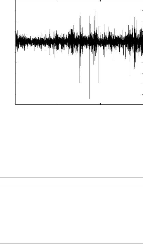
We first examine the time series of DAX daily closes from 1975 to 2005 shown
in Fig. 1.2. The daily returns δS
1d
(t) derived from the data up to 5/2000 are
shown in Fig. 5.1. At first sight, the return process looks stochastic with zero
mean. The impressive long-term growth of the DAX up to 2000 and sharp
decline thereafter, emphasized in Fig. 1.2, here show up in a small, almost in-
visible positive resp. negative mean of the return, of much smaller amplitude,
however, than the typical daily returns. We also clearly distinguish periods
with moderate (positive and negative) returns, i.e., low volatility (more fre-
quent in the first half of the time series) from periods with high (positive
and negative) returns, i.e., high volatility (more frequent in the second half
of the time series). The main question is if data like Fig. 5.1 are consistent
with a description, and to what accuracy, in terms of a simple stochastic
process with constant drift and constant volatility. Or, to the contrary, do we
have to take these parameters as time dependent, such as in the ARCH(p)
or GARCH(p,q) models of Sect. 4.4.1? Or, worse even, do the constitutive
functional relations of the stochastic process change with time?
As a first, admittedly superficial test of stationarity, we now divide the
DAX time series into seven periods of approximately equal length, and eval-
uate the average return and volatility in each period. The result of this eval-
uation is shown in Table 5.1. The central column shows the increase resp.
5.2 Stationarity of Financial Markets 103
1/1975 6/1983 11/1991 5/2000
DAX returns
−0.15
−0.10
−0.05
0.00
0.05
0.10
Fig. 5.1. Time series of daily returns of the DAX German blue chip index from 1975
to 2000. Analysis courtesy of Stephan Dresel based on data provided by Deutsche
Bank Research
Table 5.1. Average return δS
1d
(t) and volatility σ of the DAX index in
seven approximately equally long periods from January 2, 1975, to Decem-
ber 31, 2004. Analysis courtesy of Stephan Dresel based on data provided
by Deutsche Bank Research supplemented by data downloaded from Yahoo,
http://de.finance.yahoo.com
Period Return [d
−1
] Volatility [d
−1/2
]
02.01.1975–15.03.1979 0.00028 0.0071
16.03.1979–10.06.1983 0.00021 0.0078
13.06.1983–03.09.1987 0.00072 0.0104
04.09.1987–02.12.1991 0.00002 0.0155
03.12.1991–14.02.1996 0.00042 0.0091
16.02.1996–05.05.2000 0.00106 0.0149
08.05.2000–31.12.2004 −0.00049 0.0184
decrease of the average returns with time, which is responsible for the in-
creasing slope of the DAX index in Fig. 1.2. The average return increases by
a factor of three to four from 1975 to 2000, and decreases to even become
negative in the drawdown period from 2000 to 2005. The rather low value
in the fourth period is due to the October crash in 1987 right after the be-
ginning of our period, and another crash in 1991. The last column shows the
104 5. Scaling in Financial Data and in Physics
volatilities which also increase with time. The volatility is particularly big
after 2000.
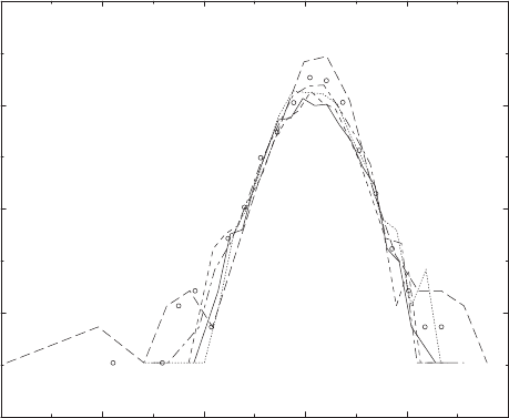
In the six periods up to May 5, 2000, we now subtract the average return
from the daily returns and then divide by the standard deviation, in order
to obtain a process with mean zero and standard deviation unity. Figure 5.2
shows the probability distributions of the returns normalized in this way, in
the six periods. Except for a few points in the wings, the six distributions do
not deviate strongly from each other. One therefore would conclude that the
rules of the stochastic process underlying financial time series do not change
with time significantly, and that most of the long-term evolution of markets
can be summarized in the time dependence of its parameters.
Notice, however, that, strictly speaking, this finding invalidates geometric
Brownian motion as a model for financial time series because µ and σ were
assumed constant there. On the other hand, if such time dependences of pa-
rameters only are important on sufficiently long time scales (which we have
not checked for the DAX data), one might take a more generous attitude,
and consider geometric Brownian motion as a candidate for the description
of the DAX on time scales which are short compared to the time scale of vari-
ations of the average returns or volatilities. Physicists take a similar attitude,
−9.0 −6.0 −3.0 0.0 3.0 6.0
normalized returns
−8.0
−6.0
−4.0
−2.0
0.0
ln P
Fig. 5.2. Probability distributions of normalized daily returns of the DAX German
blue chip index in the six equally long periods from 1975 to 2000. The normalization
procedure is explained in the text and the parameters are summarized in Table 5.1.
Solid line:period1,dotted line:period2,dashed line:period3,long-dashed line:
period 4, dot-dashed line:period5,circles: period 6. Analysis courtesy of Stephan
Dresel based on data provided by Deutsche Bank Research
5.2 Stationarity of Financial Markets 105
e.g., with temperature, in systems slightly perturbed away from equilibrium.
While being an equilibrium property in the strict sense, one may introduce
local temperatures in an inhomogeneous system on scales that are small with
respect to those over which the temperature gradients vary appreciably.
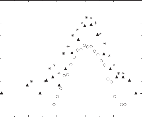
Returning to the probability distributions of the DAX returns, Fig. 5.3
shows the probability distributions of three periods (1, 4, and 6) displaced for
clarity. Period 1 is not clearly Gaussian although its tails are not very fat, a
fact that we qualitatively reproduce in periods 2 and 3. The distributions of
periods 4, 5 (not shown), and 6 do possess rather fat tails whose importance,
however, changes with time. In the DAX sample, period 4 including the
October crash in 1987, and some more turmoil in 1990 and 1991, clearly
has the fattest tails. One therefore should be extremely careful in analyzing
market data from very long periods. Markets certainly change with time, and
there may be more time dependence in financial time series than just a slow
variation of average returns and volatilities. As Fig. 5.3 suggests, even the
shape of the probability distribution might change with time.
These complications have not been studied systematically, and are ignored
in the following discussion. Depending on the underlying time scales, they
may or may not affect the conclusions of the various studies we review. We
first proceed to a critical examination of geometric Brownian motion.
−9.0 −6.0 −3.0 0.0 3.0 6.0
normalized returns
−8.0
−6.0
−4.0
−2.0
0.0
2.0
ln P
Fig. 5.3. Probability distributions (vertically displaced for clarity) of normalized
daily returns of the DAX German blue chip index in the periods 1 (open circles), 4
(filled triangles), and 6 (stars) specified in Table 5.1. Analysis courtesy of Stephan
Dresel based on data provided by Deutsche Bank Research
106 5. Scaling in Financial Data and in Physics
5.3 Geometric Brownian Motion
Geometric Brownian motion makes two fundamental hypotheses on a sto-
chastic process:
1. Successive realizations of the stochastic variable are statistically indepen-
dent.
2. Returns of financial markets, or relative changes of the stochastic vari-
able, are drawn from a normally distributed probability density func-
tion, i.e., the probability density function of the stochastic variable, resp.
prices, is log-normal.
Here, we examine these properties for financial time series.
5.3.1 Price Histories
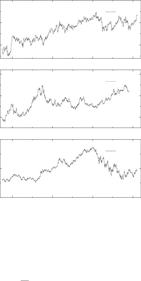
Figure 5.4 shows three financial time series which we shall use to discuss
correlations: the S&P500 index (top), the DEM/US$ exchange rate (center),
and the BUND future (bottom) [17]. The BUND future is a futures contract
on long-term German government bonds, and thereby a measure of long-term
interest-rate expectations. The data range from November 1991 to February
1995.
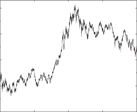
Figure 5.5 gives a chart of high-frequency data of the DAX taken on a
15-second time interval. The history is a combination of data collected in a
purpose-built database of German stock index data [59, 60] at the Depart-
ment of Physics, Bayreuth University, and data provided by an economics
database at Karlsruhe University [61].
5.3.2 Statistical Independence of Price Fluctuations
A superficial indication of statistical independence of subsequent price fluc-
tuations was given by the comparison of our numerical simulations based on
an IID random variable to the DAX time series, shown in Figs. 1.3 and 3.7.
The overall similarity between the simulation of a random walk and the daily
closing prices of the DAX would support such a hypothesis. Notice, however,
that the DAX is an index composed of 30 stocks, and correlations in the time
series of individual stocks may be lost due to averaging. Also, correlations
may well persist on time scales smaller than one day.
The question of correlations has a different emphasis for the statistician
or econometrician, and for a practitioner. Academics ask for any kind of de-
pendence in time series. Practitioners will more frequently inquire if possible
dependences can be used for generating above-average profits, and if success-
ful trading rules can be built on such correlations. Despite what has been
said in the preceding paragraph, the apparent importance of technical analy-
sis suggests that there may indeed be tradable though subtle correlations.
5.3 Geometric Brownian Motion 107
92 93 94 95
80
90
100
Bund
92 93 94 95
60
70
80
DM/$
92 93 94 95
400
450
500
S&P 500
Fig. 5.4. Three financial time series from November 1991 to February 1995: the
S&P500 index (top), the DEM/US$ exchange rate (center ), and the BUND futures
(bottom). From J.-P. Bouchaud and M. Potters: Th´eorie des Risques Financiers,
by courtesy of J.-P. Bouchaud.
c
1997 Diffusion Eyrolles (Al´ea-Saclay)
Correlation Functions
We now analyze correlation functions of returns on a fixed time scale τ,
δS
τ
(t), (5.1). The autocorrelation function of this quantity is
C
τ
(t − t
)=
1
Dτ
[δS
τ
(t) −δS
τ
(t)][δS
τ
(t
) −δS
τ
(t
)] , (5.3)
where
Dτ =var[δS
τ
(t)] , (5.4)
108 5. Scaling in Financial Data and in Physics
01.01.1999 01.07.1999 01.01.2000 01.07.2000 01.01.2001
time
4000
5000
6000
7000
8000
DAX performance index
Fig. 5.5. Chart of the DAX German blue chip index during 1999 and 2000. Data are
taken on a 15-second time scale. From S. Dresel: Modellierung von Aktienm¨arkten
durch stochastische Prozesse, Diplomarbeit, Universit¨at Bayreuth, 2001, by cour-
tesy of S. Dresel
to emphasize the similarity to diffusion. Using (5.2), we also have
C
τ
(t − t
)=δs
τ
(t)δs
τ
(t
) . (5.5)
For statistically independent data, we have C
τ
(t −t
)=0fort = t
(at least
in the limit of very large samples).
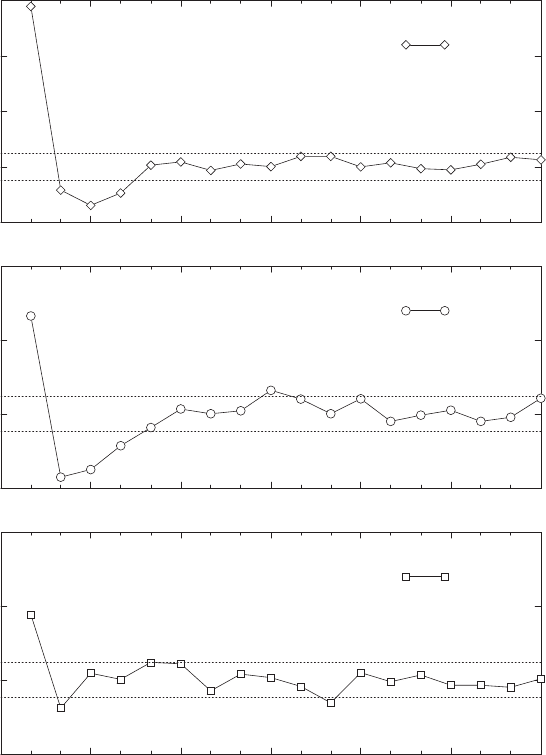
Figure 5.6 shows the autocorrelation functions of the three assets repre-
sented in Fig. 5.4 with price changes evaluated on a τ = 5-minute scale [17].
For time lags below 30 minutes, there are weak correlations above the 3σ
level. Above 30-minute time lags, correlations are not significant.
When errors are random and normally distributed (a standard assump-
tion), the standard deviation determines the confidence levels as
σ : 32%
2σ :5%
3σ :0.2%
10σ :2× 10
−23
⎫
⎪
⎪
⎬
⎪
⎪
⎭
=2
∞
Λ
P (S)dS. (5.6)
Under a null hypothesis of vanishing correlations, 32% of the data may ran-
domly lie outside a 1σ corridor, or 0.2% of the data may be outside a 3σ
corridor.
5.3 Geometric Brownian Motion 109
0 153045607590
-0.05
0.00
0.05
Bund
0 153045607590
-0.05
0.00
0.05
DEM/$
0 153045607590
-0.05
0.00
0.05
0.10
S&P 500
Fig. 5.6. Autocorrelation functions of the S&P500 index (top), the DEM/US$
exchange rate (center ), and the BUND future (bottom), over a time scale τ =5
minutes. The horizontal scale is the time separation t−t
in minutes. The horizontal
dotted lines are the 3σ confidence levels. From J.-P. Bouchaud and M. Potters:
Th´eorie des Risques Financiers, by courtesy of J.-P. Bouchaud.
c
1997 Diffusion
Eyrolles (Al´ea-Saclay)
In Fig. 5.6 for time lags above 30 minutes, the (null) hypothesis of statis-
tically independent price changes therefore cannot be rejected for the three
assets studied. The non-random deviations out of the 3σ corridor for smaller
time lags, on the other hand, indicate non-vanishing correlations in this range.
Consistent with this is the finding that no correlations significant on the 3σ
