Tsoulfanidis N. Measurement and detection of radiation

Подождите немного. Документ загружается.

418

MEASUREMENT

AND

DETECTION

RADIATION

where

linear background

step function

A(1

erf

[(x,

x)/&]}

tail function having an exponential form on the left of the peak and

a Gaussian on the right

In addition to the methods discussed so far, there are others that use mixed

technique^.^^,^^

No matter what the method is, the analysis has to be done by

computer, and numerous computer codes have been developed for that purpose.

Examples are the codes sAMPO?~ SISYPHUS-I1 and SHIITY-11: HYPER-

and GAUSS.37

The determination of the absolute intensity of a gamma requires that the

efficiency of the detector be known for the entire energy range of interest. The

efficiency is determined from information provided by the energy spectrum of

the calibration source. Using the known energy and intensity of the gammas

emitted by the source, a table is constructed giving efficiency of the detector for

the known energy peaks. The efficiency at intermediate points is obtained either

by interpolation or, better yet, by fitting an analytic form to the data of the table

(see Sec. 12.7.1).

As in the case of minimum detectable activity (Sec. 2.20), two types of errors

are encountered when one tries to identify peaks in a complex energy

spectrum.38

Type I arises when background fluctuations are falsely identified as true peaks.

Type I1 arises when fluctuations in the background obscure true peaks. Criteria

are set in the form of confidence limits (see Sec. 2.20 and Ref. 38) that can be

used to avoid both types of errors.

12.7.4 Timing Characteristics

the Pulse

For certain measurements, like coincidence-anticoincidence counting or experi-

ments involving accelerators, the time resolution of the signal is also important,

in addition to energy resolution. For timing purposes, it is essential to have

pulses with constant risetime.

No detector produces pulses with exactly the same risetime. This variation is

due to the fact that electrons are produced at different points inside the

detector volume, and thus traverse different distances before they reach the

point of their collection. As a result, the time elapsing between production of

the charge and its collection is not the same for all the carriers

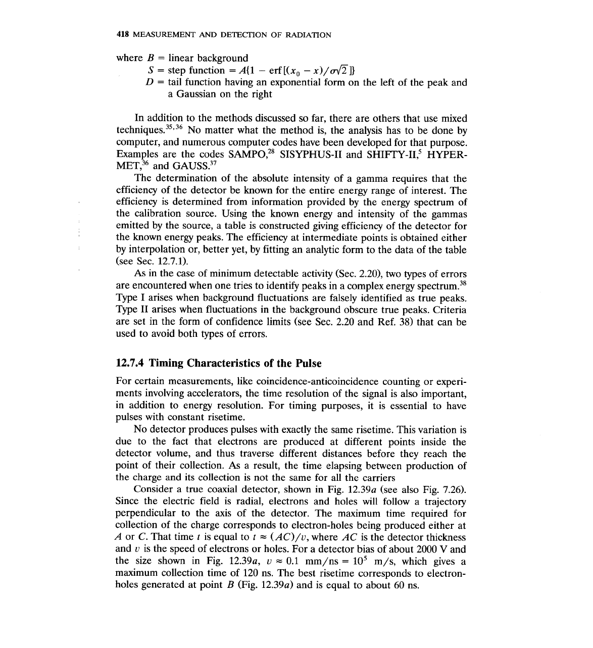
Consider a true coaxial detector, shown in Fig. 12.39~ (see also Fig. 7.26).

Since the electric field is radial, electrons and holes will follow a trajectory

perpendicular to the axis of the detector. The maximum time required for

collection of the charge corresponds to electron-holes being produced either at

A or C. That time

is equal to

(AC)/u, where AC is the detector thickness

and

is the speed of electrons or holes. For a detector bias of about 2000

and

the size shown in Fig. 12.39a,

0.1 mm/ns

lo5

m/s, which gives a

maximum collection time of 120 ns. The best risetime corresponds to electron-

holes generated at point

(Fig. 12.39~) and is equal to about 60 ns.

PHOTON

(GAMMA-RAY

AND

X-RAY)

SPECTROSCOPY

419

Figure

1239

(a)

In a true coaxial detector, electrons and holes travel along the direction ABC.

(b)

In wrap-around coaxial detectors, the carriers may travel along ABC but also along the longer path

A'B'C'.

The pulse risetime is essentially equal to the collection time. For the

detector shown in Fig. 12.39a, the risetime will vary between 60 and 120 ns. For

other detector geometries the variation in

risetime is greater because the

electrons and holes, following the electric field lines, may travel distances larger

than the thickness of the detector core (Fig. 12.396). The variation in

risetime

for the detector of Fig. 12.396 will be between 60 and 200 ns. The distribution of

pulse risetimes for commercial detectors is a bell-type curve, not exactly Gauss-

ian, with a FWHM of less than 5 ns.

12.8

CdTe AND

HgI,

DETECTORS AS

GAMMA

SPECTROMETERS

A great advantage for CdTe and HgI,

detector^,^^-^^

compared to Ge and Si(Li)

detectors, is that they can operate at room temperature (see also Sec. 7.5.6). At

this time, they can be obtained in relatively small volumes, but they still have an

intrinsic efficiency of about 75 percent at 100 keV because of the high atomic

number of the elements involved. The energy resolution of CdTe detectors is 18

percent at 6

keV and 1.3 percent at 662 keV. The corresponding numbers for

HgI, are

percent and 0.7 percent.45

The HgI, detectors are very useful for the measurement for X-rays with

energy less than 10

keV. In that energy range, resolutions of 245 eV at 1.25

ke~~~ and 295 eV at 5.9 kevso have been reported.

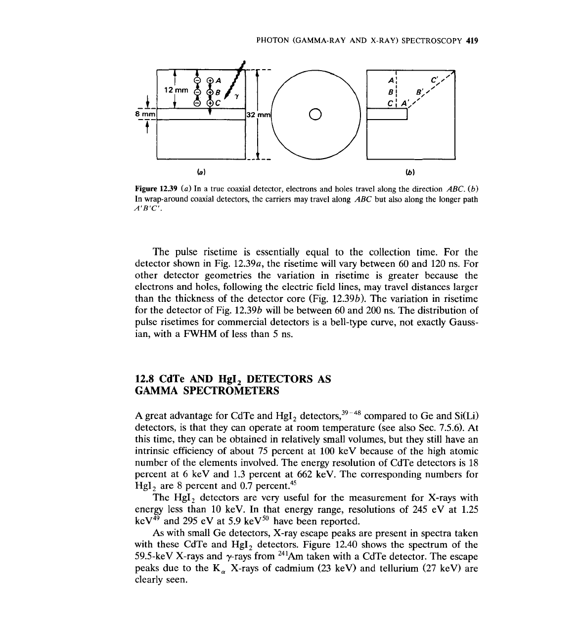
As with small Ge detectors, X-ray escape peaks are present in spectra taken

with these CdTe and HgI, detectors. Figure 12.40 shows the spectrum of the

59.5-keV X-rays and y-rays from 241~rn taken with a CdTe detector. The escape

peaks due to the

X-rays of cadmium (23 keV) and tellurium (27 keV) are

clearly seen.

420

MEASUREMENT

AND

DETECTION

RADIATION

13.9

keV

14'

Am source

10.000

CdTe

DET

02905

17.7

keV

7i=~d=2@

Pulser

Channel number

Figure

12.40

The 59.5-keV

X-ray

241~m

detected with

CdTe detector

(from

Ref.

42).

12.9

DETECTION OF

X-RAYS

WITH

Si(Li)

DETECTOR

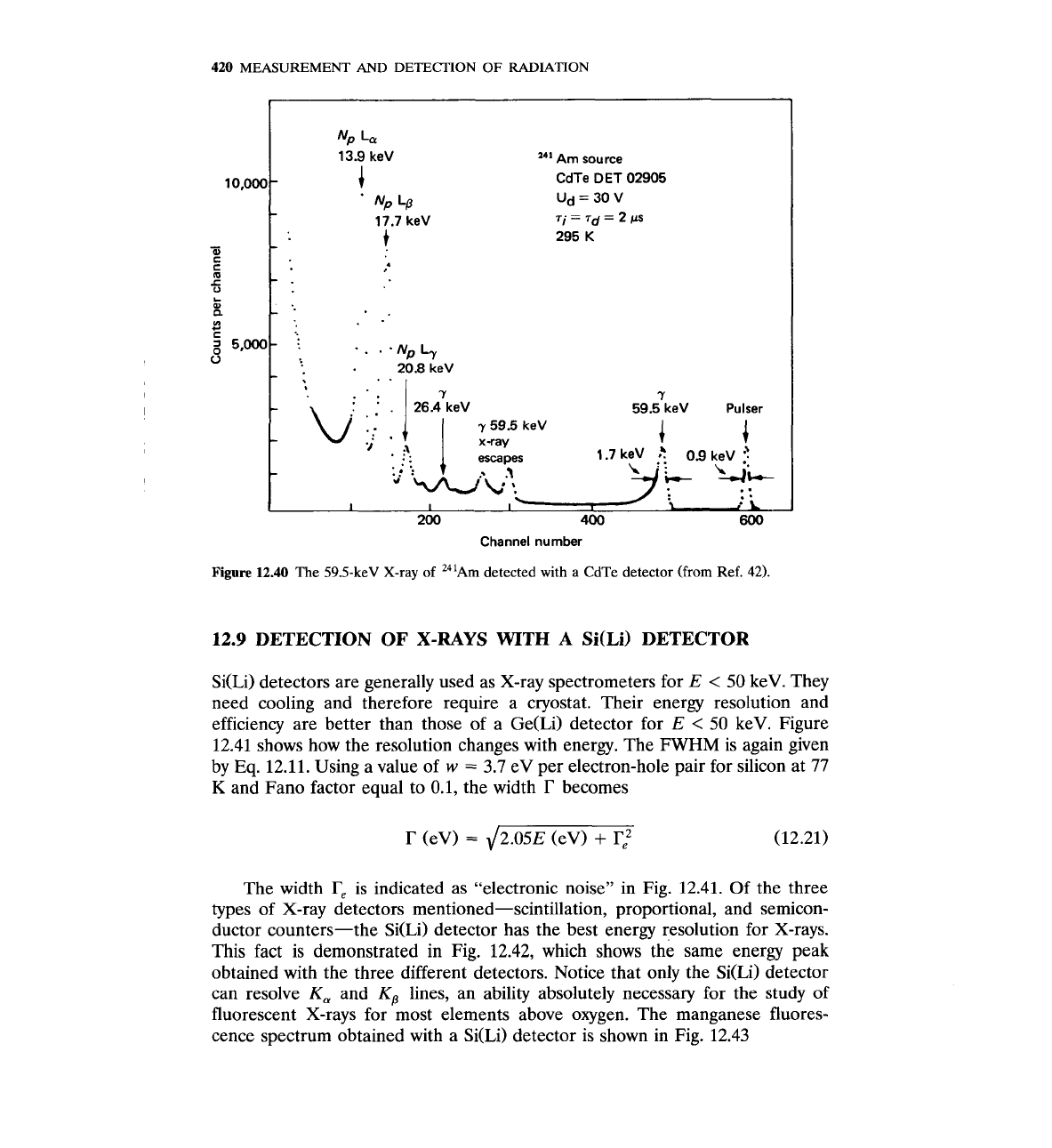
Si(Li) detectors are generally used as X-ray spectrometers for

keV. They

need cooling and therefore require a cryostat. Their energy resolution and

efficiency are better than those of a Ge(Li) detector for

keV. Figure

12.41 shows how the resolution changes with energy. The FWHM is again given

by Eq. 12.11. Using a value of

3.7 eV per electron-hole pair for silicon at 77

and Fano factor equal to 0.1, the width

becomes

The width

is indicated as "electronic noise" in Fig. 12.41. Of the three

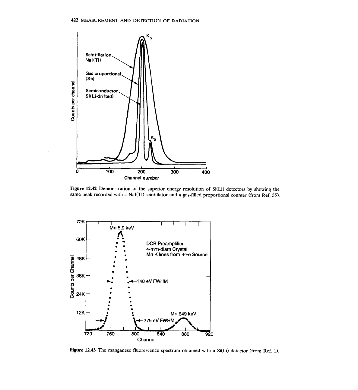
types of X-ray detectors mentioned-scintillation, proportional, and semicon-

ductor counters-the Si(Li) detector has the best energy resolution for X-rays.

This fact is demonstrated

Fig. 12.42, which shows the same energy peak

obtained with the three different detectors. Notice that only the Si(Li) detector

can resolve

and

lines, an ability absolutely necessary for the study of

fluorescent X-rays for most elements above oxygen. The manganese fluores-

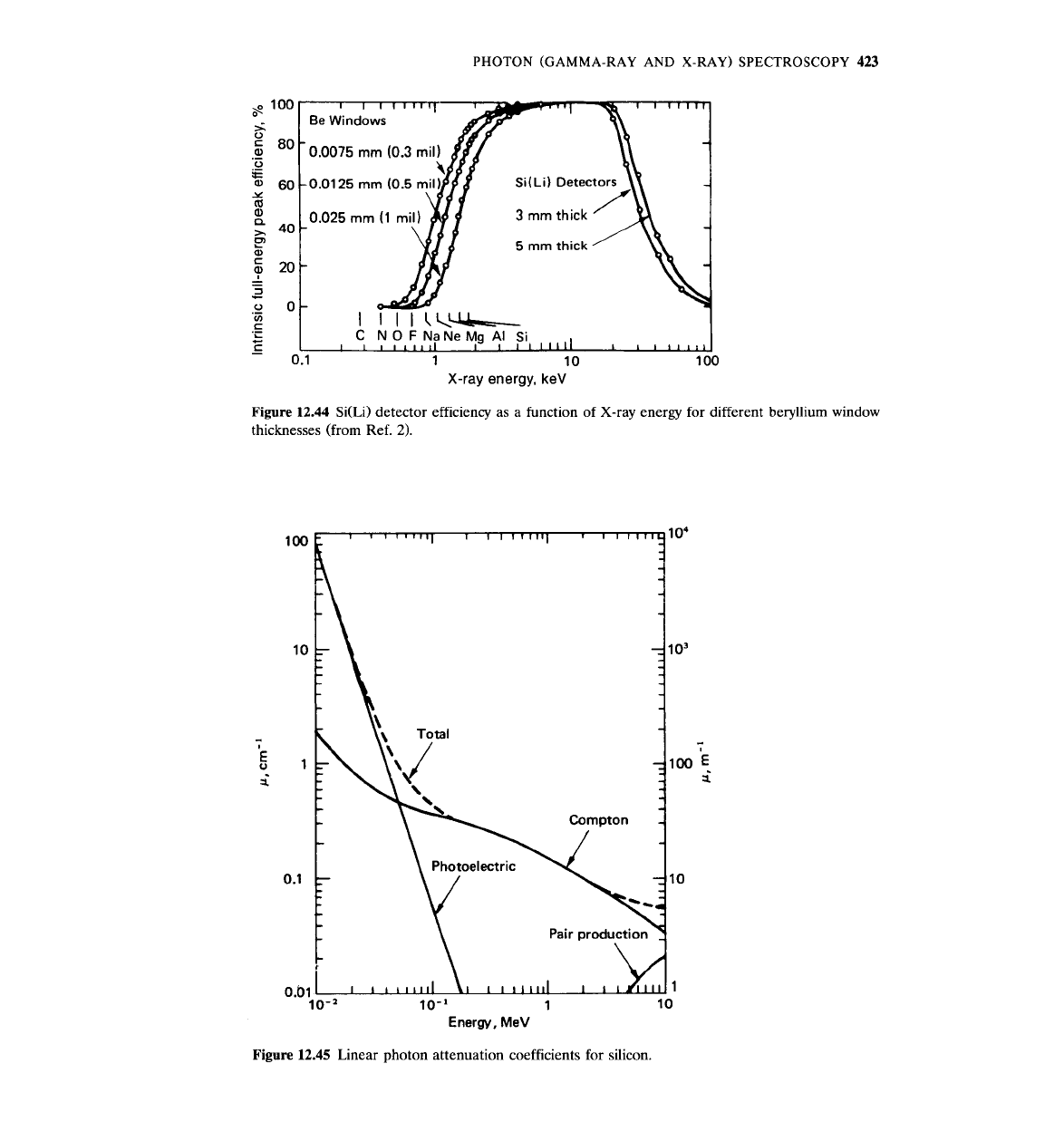
cence spectrum obtained with a Si(Li) detector is shown in Fig. 12.43

PHOTON

(GAMMA-RAY AND

X-RAY)

SPECTROSCOPY

421

FWHM (eV)

J(FwHM);,~,,

r2.35

JFEWI

- -

Electronic noise

1,000

-10

keV

Photon energy(eV1

(average energy to create

holeelectron pair at

temperature)

1111

111111

11111111

Ill&

0.1 1

10 100

~,OOo

keV

Figure

12.41

Si(Li) detector energy resolution as a function of X-ray energy (from Ref.

2).

What is

indicated as electronic noise is the width

re.

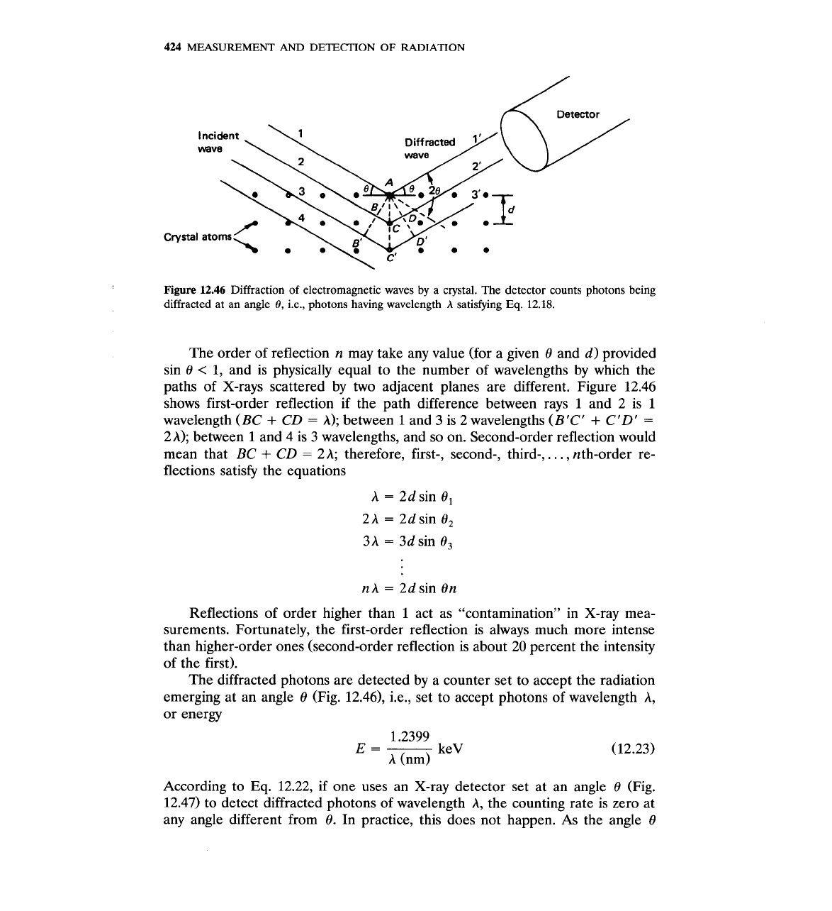
The dependence of Si(Li) detector efficiency on the X-ray energy is shown

in Fig. 12.44. For

keV, the efficiency drops because of absorption of the

incident X-rays by the beryllium detector window. For

15 keV, the effi-

ciency falls off because of the decrease of the total linear attenuation coefficient

of X-rays in silicon (Fig. 12.45).

12.10

DETECTION OF X-RAYS WITH

CRYSTAL

SPECTROMETER

The measurement of X-ray energy by wavelength-dispersive crystal spectrome-

ters is based on the phenomenon of diffraction of electromagnetic waves from a

crystal (see Compton and Allison, and Cullity). Consider an X-ray of wavelength

incident at an angle

on a crystal with interplanar spacing d (Fig. 12.46). The

incident X-rays will be scattered by the atoms of the crystal in all directions, but

result of the periodicity of the atom positions, there are certain directions

along which constructive interference of the scattered photons takes place. The

direction of constructive interference of the diffracted beam is given by the

Bragg condition

2dsin

(12.22)

where n is the order of reflection

(

1,2,3,.

. .

Equation 12.22 states that for

constructive interference, the path difference between any two rays (photons)

must be an integral number of wavelengths. In Fig. 12.46, the path difference for

rays

and 2 is

2dsin

422

MEASUREMENT

AND

DETECTION OF RADIATION

Semiconductor

100

200

300 400

Channel number

Figure 12.42 Demonstration of the superior energy resolution of Si(Li) detectors by showing the

same peak recorded with a NaI(TI) scintillator and a gas-filled proportional counter (from Ref. 55).

6OK

. DCR Preamplifier

. 4-mm-diam Crystal

lines

from

+Fe

Source

.+I48 eV

FWHM

M n 649 keV

Channel

Figure 12.43 The manganese fluorescence spectrum obtained with a Si(Li) detector (from Ref.

1).

PHOTON (GAMMA-RAY AND X-RAY) SPECTROSCOPY 423

X-ray energy, keV

Figure

12.44

Si(Li) detector efficiency as a function of X-ray energy for different beryllium window

thicknesses (from Ref.

2).

Energy,

MeV

Figure

12.45 Linear photon attenuation coefficients for silicon.

424

MEASUREMENT

AND

DETECTION

RADIATION

Figure

12.46

Diffraction of electromagnetic waves

a crystal. The detector counts photons being

diffracted at an angle

i.e., photons having wavelength

satisfying

Eq.

12.18.

The order of reflection n may take any value (for a given

and d) provided

sin 8

and is physically equal to the number of wavelengths by which the

paths of X-rays scattered by two adjacent planes are different. Figure 12.46

shows first-order reflection if the path difference between rays

and 2 is

wavelength (BC

A); between

and 3 is 2 wavelengths (B'C'

C'D'

A); between

and 4 is 3 wavelengths, and so on. Second-order reflection would

mean that

A; therefore, first-, second-, third-,

. . .

nth-order re-

flections satisfy the equations

2dsin

2d sin

3d sin

2d sin On

Reflections of order higher than

act as "contamination" in X-ray mea-

surements. Fortunately, the first-order reflection is always much more intense

than higher-order ones (second-order reflection is about 20 percent the intensity

of the first).

The diffracted photons are detected by a counter set to accept the radiation

emerging at an angle

(Fig. 12.46), i.e., set to accept photons of wavelength A,

or energy

According to

Eq.

12.22, if one uses an X-ray detector set at an angle

(Fig.

12.47) to detect diffracted photons of wavelength A, the counting rate is zero at

any angle different from 8. In practice, this does not happen. As the angle

PHOTON

(GAMMA-RAY

AND

X-RAY) SPECTROSCOPY

425

changes from rotating the crystal around an axis perpendicular to the plane

formed by the incident and diffracted beams, the counting rate of the detector

will have a maximum at 8

00,

where

sin O,, but it will gradually go to

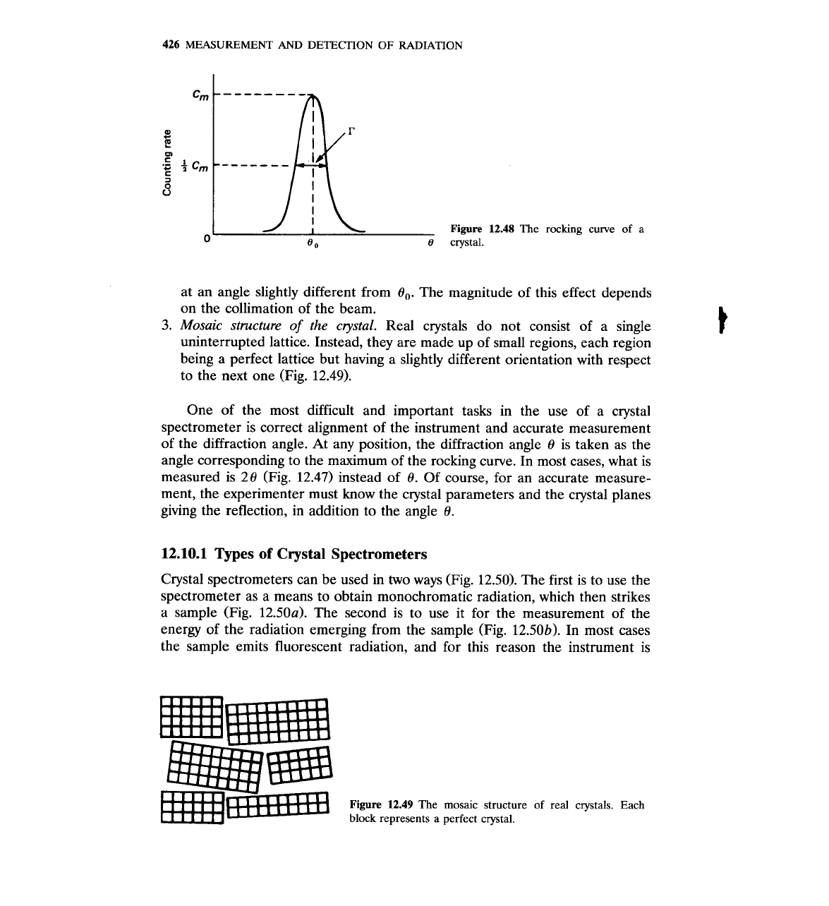
zero as shown in Fig. 12.48. The curve of Fig. 12.48, known as the

rocking curve

of the crystal, is the result of incomplete destructive interference of the

diffracted X-rays. The rocking curve is the equivalent of the Gaussian response

function of a detector to a monoenergetic photon source. However, its origin is

not statistical, as the following discussion shows.

As stated earlier, the Bragg condition

(Eq.

12.22) indicates that the waves

(photons) scattered by the different crystal planes have a path difference equal

to an integral number of wavelengths along the direction

satisfying Eq. 12.22.

But what if the angle 8 is such that the path difference is only a fraction of a

wavelength? The destructive interference of the scattered waves is not complete

and the result is radiation of lower amplitude. This partial constructive interfer-

ence may happen because of three reasons:

Finite thickness of the clystal.

crystal with finite thickness consists of a finite

number of planes. For any angle O,, there are planes with no matching

partner to create the correct phase difference in scattered radiation for

complete destructive interference. The width

of the rocking curve, due to

the finite thickness of the crystal, is given by (see Cullity)

where

is the crystal thickness. Notice that

depends on the wavelength,

the thickness, and the diffraction angle. If

mm, the width

negligible for the cases encountered in practice.

2. Nonparallel incident rays.

It is impossible to produce a beam consisting of

exactly parallel rays. Thus, at any angle 8, there are X-rays hitting the crystal

ncident wave

with wavelength

Detector

Crystal

Figure

12.47

The rocking curve of the c~ystal

.\.

is obtained by rotating the crystal

and

keep-

ing source and detector fixed.

426

MEASUREMENT

AND

DETECTION OF RADIATION

Figure

crystal.

12.48

The

rocking

at an angle slightly different from

8,.

The magnitude of this effect depends

on the collimation of the beam.

Mosaic structure of the cystal.

Real crystals do not consist of a single

uninterrupted lattice. Instead, they are made up of small regions, each region

being a perfect lattice but having a slightly different orientation with respect

to the next one (Fig.

12.49).

One of the most difficult and important tasks in the use of a crystal

spectrometer is correct alignment of the instrument and accurate measurement

of the diffraction angle. At any position, the diffraction angle

is taken as the

angle corresponding to the maximum of the rocking curve. In most cases, what is

measured is

(Fig.

12.47)

instead of

Of course, for an accurate measure-

ment, the experimenter must know the crystal parameters and the crystal planes

giving the reflection, in addition to the angle

12.10.1

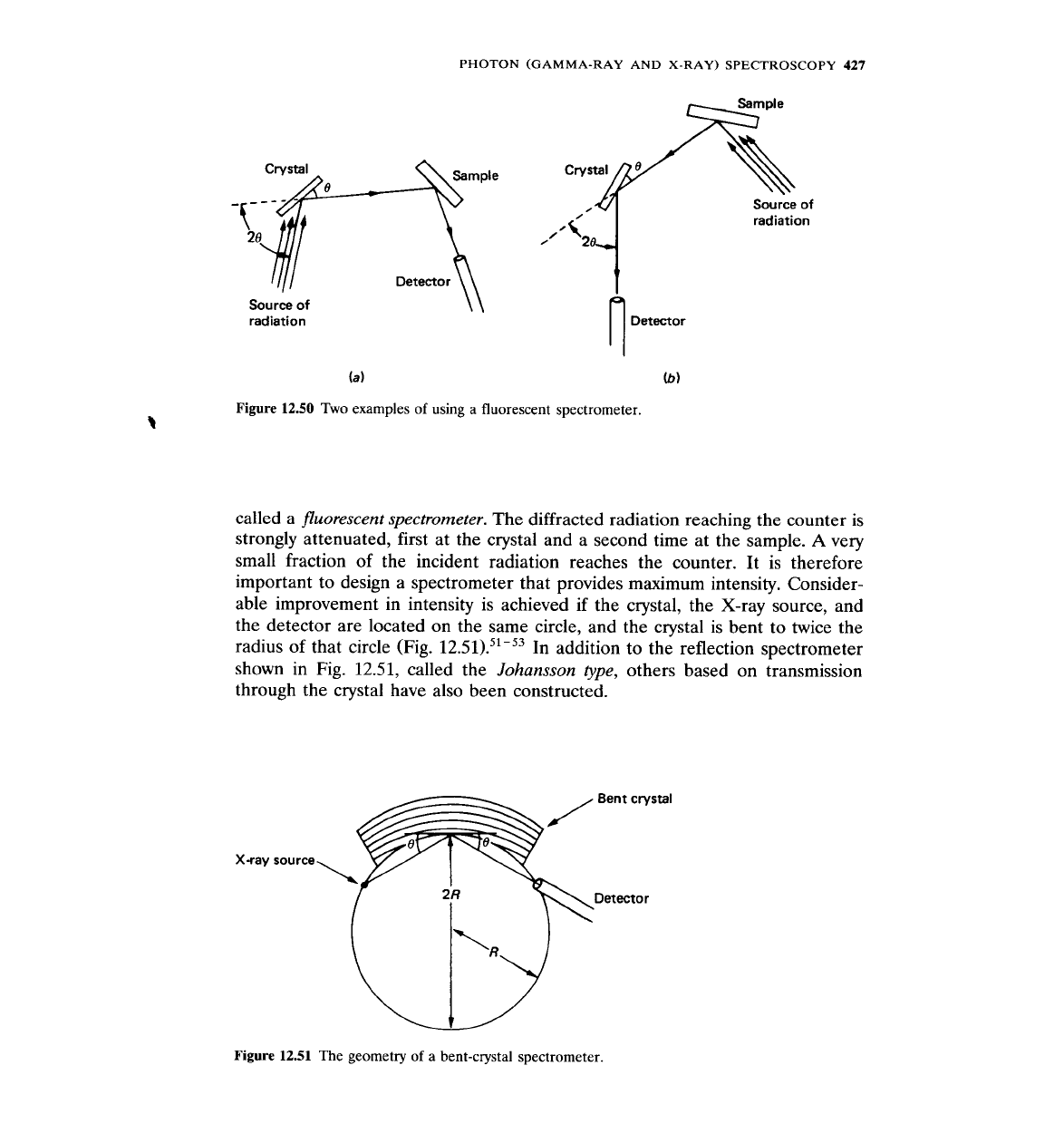
Types of Crystal Spectrometers

Crystal spectrometers can be used in two ways (Fig.

12.50).

The first is to use the

spectrometer as a means to obtain monochromatic radiation, which then strikes

a sample (Fig.

12.50a).

The second is to use it for the measurement of the

energy of the radiation emerging from the sample (Fig.

12.50b).

In most cases

the sample emits fluorescent radiation, and for this reason the instrument is

Figure

12.49

The mosaic structure of real crystals. Each

block represents a perfect crystal.

PHOTON

(GAMMA-RAY AND X-RAY)

SPECTROSCOPY

427

Crystal

Detector

Source of

radiation

Crystal

radiation

Detector

(a)

(6)

Figure

12.50

Two examples of using a fluorescent spectrometer.

called a

fluorescent spectrometer.

The diffracted radiation reaching the counter is

strongly attenuated, first at the crystal and a second time at the sample.

very

small fraction of the incident radiation reaches the counter. It is therefore

important to design a spectrometer that provides maximum intensity. Consider-

able improvement in intensity is achieved if the crystal, the X-ray source, and

the detector are located on the same circle, and the crystal is bent to twice the

radius of that circle (Fig.

12.51).~l-'~

In addition to the reflection spectrometer

shown in Fig.

12.51,

called the

Johansson

type,

others based on transmission

through the crystal have also been constructed.

X-ray source

Figure

12.51

The geometry

a bent-crystal spectrometer.