Trauth M.H., MATLAB® Recipes for Earth Sciences, Third edition

8 1 DATA ANALYSIS IN EARTH SCIENCES

Spatial analysis• –  is is the analysis of parameters in 2D or 3D space

and hence two or three of the required parameters are coordinate num-

bers.  ese methods include descriptive tools to investigate the spatial

pattern of geographically distributed data. Other techniques involve

spatial regression analysis to detect spatial trends. Also included are 2D

and 3D interpolation techniques, which help to estimate surfaces repre-

senting the predicted continuous distribution of the variable throughout

the area. Examples are drainage-system analysis, the identi cation of old

landscape forms and lineament analysis in tectonically active regions.

Image processing• –  e processing and analysis of images has become in-

creasingly important in earth sciences.  ese methods involve importing

and exporting, compressing and decompressing, and displaying images.

Image processing also aims to enhance images for improved intelligibil-

ity, and to manipulate images in order to increase the signal-to-noise ra-

tio. Advanced techniques are used to extract speci c features, or analyze

shapes and textures, such as for counting mineral grains or fossils in mi-

croscope images. Another important application of image processing is

in the use of satellite remote sensing to map certain types of rocks, soils

and vegetation, as well as other parameters such as soil moisture, rock

weathering and erosion.

Multivariate analysis• –  ese methods involve the observation and

analysis of more than one statistical variable at a time. Since the graphi-

cal representation of multidimensional data sets is di cult, most of these

methods include dimension reduction. Multivariate methods are widely

used on geochemical data, for instance in tephrochronology, where volca-

nic ash layers are correlated by geochemical  ngerprinting of glass shards.

Another important usage is in the comparison of species assemblages in

ocean sediments for the reconstruction of paleoenvironments.

Analysis of directional data• – Methods to analyze circular and spherical

data are widely used in earth sciences. Structural geologists measure and

analyze the orientation of slickensides (or striae) on a fault plane, circular

statistical methods are common in paleomagnetic studies, and micro-

structural investigations include the analysis of grain shapes and quartz

c-axis orientations in thin sections.

Some of these methods of data analysis require the application of numeri-

cal methods such as interpolation techniques. While the following text

Recommended Reading

Borradaile G (2003) Statistics of Earth Science Data –  eir Distribution in Time, Space

and Orientation. Springer, Berlin Heidelberg New York

Carr JR (1994) Numerical Analysis for the Geological Sciences. Prentice Hall, Englewood

Cli s, New Jersey

Davis JC (2002) Statistics and Data Analysis in Geology,  ird Edition. John Wiley and

Sons, New York

Gonzalez RC, Woods RE, Eddins SL (2009) Digital Image Processing Using MATLAB –

2nd Edition. Gatesmark Publishing, LLC

Hanneberg WC (2004) Computational Geosciences with Mathematica. Springer, Berlin

Heidelberg New York

Holzbecher E (2007) Environmental Modeling using MATLAB. Springer, Berlin Heidelberg

New York

Middleton GV (1999) Data Analysis in the Earth Sciences Using MATLAB. Prentice Hall,

New Jersey

Press WH, Teukolsky SA, Vetterling WT, Flannery BP (2007) Numerical Recipes:  e Art

of Scienti c Computing – 3rd Edition. Cambridge University Press, Cambridge

Swan ARH, Sandilands M (1995) Introduction to Geological Data Analysis. Blackwell

Sciences, Oxford

2 INTRODUCTION TO MATLAB

2 Introduction to MATLAB

2.1 MATLAB in Earth Sciences

MATLAB

is a so ware package developed by The MathWorks Inc., found-

ed by Cleve Moler, Jack Little and Steve Bangert in 1984, which has its head-

quarters in Natick, Massachusetts (http://www.mathworks.com). MATLAB

was designed to perform mathematical calculations, to analyze and visual-

ize data, and to facilitate the writing of new so ware programs.  e advan-

tage of this so ware is that it combines comprehensive math and graphics

functions with a powerful high-level language. Since MATLAB contains a

large library of ready-to-use routines for a wide range of applications, the

user can solve technical computing problems much more quickly than with

traditional programming languages, such as C++ and FORTRAN.  e

standard library of functions can be signi cantly expanded by add-on tool-

boxes, which are collections of functions for special purposes such as image

processing, creating map displays, performing geospatial data analysis or

solving partial di erential equations.

During the last few years, MATLAB has become an increasingly popu-

lar tool in earth sciences. It has been used for  nite element modeling, pro-

cessing of seismic data, analyzing satellite imagery, and for the generation of

digital elevation models from satellite data.  e continuing popularity of the

so ware is also apparent in published scienti c literature, and many confer-

ence presentations have also made reference to MATLAB. Universities and

research institutions have recognized the need for MATLAB training for

sta and students, and many earth science departments across the world now

o er MATLAB courses for undergraduates. The MathWorks Inc. provides

classroom kits for teachers at a reasonable price, and it is also possible for

students to purchase a low-cost edition of the so ware.  is student version

provides an inexpensive way for students to improve their MATLAB skills.

 e following sections contain a tutorial-style introduction to MATLAB,

to the setup on the computer (Section 2.2), the syntax (Section 2.3), data

M.H. Trauth, MATLAB

Recipes for Earth Sciences, 3rd ed.,

DOI 10.1007/978-3-642-12762-5_2, © Springer-Verlag Berlin Heidelberg 2010

12 2 INTRODUCTION TO MATLAB

input and output (Sections 2.4 and 2.5), programming (Section 2.6), and

visualization (Section 2.7). Advanced sections are also included on gener-

ating M- les to regenerate graphs (Section 2.8) and on publishing M- les

(Section 2.9). It is recommended to go through the entire chapters in order

to obtain a good knowledge of the so ware before proceeding to the follow-

ing chapter. A more detailed introduction can be found in the MATLAB 7

Getting Started Guide ( e MathWorks 2010) which is available in print

form, online and as PDF  le.

In this book we use MATLAB Version 7.10 (Release 2010a), the Image

Processing Toolbox Version 7.0, the Mapping Toolbox Version 3.1, the Signal

Processing Toolbox Version 6.13, the Statistics Toolbox Version 7.3 and the

Wavelet Toolbox Version 4.5.

2.2 Getting Started

 e so ware package comes with extensive documentation, tutorials and

examples.  e  rst three chapters of the book MATLAB 7 Getting Started

Guide ( e MathWorks 2010) are directed at beginners.  e chapters on

programming, creating graphical user interfaces (GUI) and development

environments are aimed at more advanced users. Since MATLAB 7 Getting

Started Guide provides all the information required to use the so ware,

this introduction concentrates on the most relevant so ware components

and tools used in the following chapters of this book.

A er the installation of MATLAB, the so ware is launched either by

clicking the shortcut icon on the desktop or by typing

matlab

in the operating system prompt.  e so ware then comes up with several

window panels (Fig. 2.1).  e default desktop layout includes the Current

Folder panel that lists the  les in the directory currently being used.  e

Command Window presents the interface between the so ware and the

user, i. e., it accepts MATLAB commands typed a er the prompt,

>>.  e

Workspace panel lists the variables in the MATLAB workspace, which is

empty when starting a new so ware session.  e Command History panel

records all operations previously typed into the Command Window and en-

ables them to be recalled by the user. In this book we mainly use the Command

Window and the built-in Editor, which can be launched by typing

2.2 GETTING STARTED 13

2 INTRODUCTION TO MATLAB

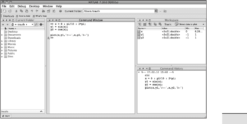
Fig. 2.1 Screenshot of the MATLAB default desktop layout including the Current Folder

(le in the  gure), the Command Window (center), the Workspace (upper right) and

Command History (lower right) panels.  is book uses only the Command Window and

the built-in Editor, which can be called up by typing edit a er the prompt. All information

provided by the other panels can also be accessed through the Command Window.

edit

or by selecting the Editor from the Desktop menu. By default, the so -

ware stores all of your MATLAB-related  les in the startup folder named

MATLAB. Alternatively, you can create a personal working directory in

which to store your MATLAB-related  les. You should then make this new

directory the working directory using the Current Folder panel or the

Folder Browser at the top of the MATLAB desktop.  e so ware uses a

search path to  nd MATLAB-related  les, which are organized in directo-

ries on the hard disk.  e default search path includes only the MATLAB

directory that has been created by the installer in the applications folder and

the default working directory. To see which directories are in the search path

or to add new directories, select Set Path from the File menu, and use the

Set Path dialog box.  e modi ed search path is saved in a  le pathdef.m

on your hard disk.  e so ware will then in future read the contents of this

 le and direct MATLAB to use your custom path list.

14 2 INTRODUCTION TO MATLAB

2.3 The Syntax

 e name MATLAB stands for matrix laboratory.  e classic object han-

dled by MATLAB is a matrix, i. e., a rectangular two-dimensional array

of numbers. A simple 1-by-1 matrix or array is a scalar. Matrices with one

column or row are vectors, time series or other one-dimensional data  elds.

An m-by-n matrix or array can be used for a digital elevation model or a

grayscale image. Red, green and blue (RGB) color images are usually stored

as three-dimensional arrays, i. e., the colors red, green and blue are repre-

sented by an m-by-n-by-3 array.

Before proceeding, we need to clear the workspace by typing

clear

a er the prompt in the Command Window. Clearing the workspace is al-

ways recommended before working on a new MATLAB project. Entering

matrices or arrays in MATLAB is easy. To enter an arbitrary matrix, type

A = [2 4 3 7; 9 3 -1 2; 1 9 3 7; 6 6 3 -2]

which  rst de nes a variable A, then lists the elements of the matrix in

square brackets.  e rows of

A are separated by semicolons, whereas the ele-

ments of a row are separated by blank spaces, or alternatively, by commas.

A er pressing return, MATLAB displays the matrix

A =

2 4 3 7

9 3 -1 2

1 9 3 7

6 6 3 -2

Displaying the elements of A could be problematic for very large matrices,

such as digital elevation models consisting of thousands or millions of ele-

ments. To suppress the display of a matrix or the result of an operation in

general, the line should be ended with a semicolon.

A = [2 4 3 7; 9 3 -1 2; 1 9 3 7; 6 6 3 -2];

 e matrix A is now stored in the workspace and we can carry out some

basic operations with it, such as computing the sum of elements,

sum(A)

which results in the display

2.3 THE SYNTAX 15

2 INTRODUCTION TO MATLAB

ans =

18 22 8 14

Since we did not specify an output variable, such as A for the matrix entered

above, MATLAB uses a default variable

ans, short for answer or most re-

cent answer, to store the results of the calculation. In general, we should

de ne variables since the next computation without a new variable name

will overwrite the contents of

ans.

 e above example illustrates an important point about MATLAB: the

so ware prefers to work with the columns of matrices.  e four results of

sum(A) are obviously the sums of the elements in each of the four columns

A. To sum all elements of A and store the result in a scalar b, we simply

need to type

b = sum(sum(A));

which  rst sums the columns of the matrix and then the elements of the re-

sulting vector. We now have two variables,

A and b, stored in the workspace.

We can easily check this by typing

whos

which is one the most frequently-used MATLAB commands.  e so -

ware then lists all variables in the workspace, together with information

about their sizes or dimensions, number of bytes, classes and attributes (see

Section 2.5 for details about classes and attributes of objects).

Name Size Bytes Class Attributes

A 4x4 128 double

ans 1x4 32 double

b 1x1 8 double

Note that by default MATLAB is case sensitive, i. e., A and a can de ne two

di erent variables. In this context, it is recommended that capital letters be

used for matrices and lower-case letters for vectors and scalars. We could

now delete the contents of the variable

ans by typing

clear ans

Next, we will learn how speci c matrix elements can be accessed or ex-

changed. Typing

A(3,2)

simply yields the matrix element located in the third row and second col-

umn, which is

9.  e matrix indexing therefore follows the rule (row, col-

16 2 INTRODUCTION TO MATLAB

umn). We can use this to replace single or multiple matrix elements. As an

example, we type

A(3,2) = 30

to replace the element A(3,2) by 30 and to display the entire matrix.

A =

2 4 3 7

9 3 -1 2

1 30 3 7

6 6 3 -2

If we wish to replace several elements at one time, we can use the colon

operator. Typing

A(3,1:4) = [1 3 3 5]

A(3,:) = [1 3 3 5]

replaces all elements of the third row of the matrix A.  e colon operator

also has several other uses in MATLAB, for instance as a shortcut for enter-

ing matrix elements such as

c = 0 : 10

which creates a row vector containing all integers from 0 to 10.  e resultant

MATLAB response is

c =

0 1 2 3 4 5 6 7 8 9 10

Note that this statement creates 11 elements, i. e., the integers from 1 to 10

and the zero. A common error when indexing matrices is to ignore the zero

and therefore expect 10 elements instead of 11 in our example. We can check

this from the output of

whos.

Name Size Bytes Class Attributes

A 4x4 128 double

ans 1x1 8 double

b 1x1 8 double

c 1x11 88 double

 e above command creates only integers, i. e., the interval between the vec-

tor elements is one unit. However, an arbitrary interval can be de ned, for

example 0.5 units.  is is later used to create evenly-spaced time axes for

2.3 THE SYNTAX 17

2 INTRODUCTION TO MATLAB

time series analysis. Typing

c = 1 : 0.5 : 10

results in the display

c =

Columns 1 through 6

1.0000 1.5000 2.0000 2.5000 3.0000 3.5000

Columns 7 through 12

4.0000 4.5000 5.0000 5.5000 6.0000 6.5000

Columns 13 through 18

7.0000 7.5000 8.0000 8.5000 9.0000 9.5000

Column 19

10.0000#

which autowraps the lines that are longer than the width of the Command

Window.  e display of the values of a variable can be interrupted by press-

ing Ctrl+C ( Control+C) on the keyboard.  is interruption a ects only

the output in the Command Window, whereas the actual command is pro-

cessed before displaying the result.

MATLAB provides standard arithmetic operators for addition,

+, and

subtraction,

-.  e asterisk, *, denotes matrix multiplication involving in-

ner products between rows and columns. For instance, we multiply the ma-

trix

A with a new matrix B

B = [4 2 6 5; 7 8 5 6; 2 1 -8 -9; 3 1 2 3];

the matrix multiplication is then

C = A * B'

where ' is the complex conjugate transpose, which turns rows into columns

and columns into rows.  is generates the output

C =

69 103 -79 37

46 94 11 34

75 136 -76 39

44 93 12 24

In linear algebra, matrices are used to keep track of the coe cients of linear

transformations.  e multiplication of two matrices represents the combi-

nation of two linear transformations into a single transformation. Matrix

multiplication is not commutative, i. e.,

A*B' and B*A' yield di erent re-

sults in most cases. Similarly, MATLAB allows matrix divisions, right,

and le ,

\, representing di erent transformations. Finally, the so ware also

allows powers of matrices,

Trauth M.H., MATLAB® Recipes for Earth Sciences, Third edition

Подождите немного. Документ загружается.