Trauth M.H., MATLAB® Recipes for Earth Sciences, Third edition
Подождите немного. Документ загружается.

48 3 UNIVARIATE STATISTICS
skewness(corg)
ans =
-0.2529
Finally, the peakedness of the distribution is described by the kurtosis. e
result from the function
kurtosis,
kurtosis(corg)
ans =
2.4670
suggests that our distribution is slightly atter than a Gaussian distribution
since its kurtosis is lower than three.
Most of these functions have corresponding versions for data sets con-
taining gaps, such as
nanmean and nanstd, which treat NaNs as missing
values. To illustrate the use of these functions we introduce a gap into our
data set and compute the mean using
mean and nanmean for comparison.
corg(25,1) = NaN;
mean(corg)
ans =
NaN
nanmean(corg)
ans =
12.3371
In this example the function mean follows the rule that all operations with
NaNs result in NaNs, whereas the function nanmean simply skips the miss-
ing value and computes the mean of the remaining data.
As a second example, we now explore a data set characterized by a sig-
ni cant skew. e data represent 120 microprobe analyses on glass shards
hand-picked from a volcanic ash. e volcanic glass has been a ected by
chemical weathering at an initial stage, and the shards therefore exhibit
glass hydration and sodium depletion in some sectors. We can study the
distribution of sodium (in wt %) in the 120 analyses using the same proce-
dure as above. e data are stored in the le sodiumcontent_one.txt.
clear
sodium = load('sodiumcontent_one.txt');
As a rst step, it is always recommended to display the data as a histogram.

3.3 EXAMPLE OF EMPIRICAL DISTRIBUTIONS 49
3 UNIVARIATE STATISTICS
e square root of 120 suggests 11 classes, and we therefore display the data
by typing
hist(sodium,11)
[n,v] = hist(sodium,11)
n =
Columns 1 through 10
3 3 5 2 6 8 15 14 22 29
Column 11
13
v =
Columns 1 through 6
2.6738 3.1034 3.5331 3.9628 4.3924 4.8221
Columns 7 through 11
5.2518 5.6814 6.1111 6.5407 6.9704
Since the distribution has a negative skew, the mean, the median and the
mode di er signi cantly from each other.
mean(sodium)
ans =
5.6628
median(sodium)
ans =
5.9741
v(find(n == max(n)))
ans =
6.5407
e mean of the data is lower than the median, which is in turn lower than
the mode. We can observe a strong negative skewness, as expected from our
data.
skewness(sodium)
ans =
-1.1086
We now introduce a signi cant outlier to the data and explore its e ect on
the statistics of the sodium content. For this we will use a di erent data set,
which is better suited for this example than the previous data set. e new
data set contains higher sodium values of around 17 wt % and is stored in
the le sodiumcontent_two.txt.
50 3 UNIVARIATE STATISTICS
clear
sodium = load('sodiumcontent_two.txt');
is data set contains only 50 measurements, in order to better illustrate
the e ects of an outlier. We can use the same script used in the previous
example to display the data in a histogram with seven classes and compute
the number of observations
n with respect to the classes v.
[n,v] = hist(sodium,7);
mean(sodium)
ans =
16.6379
median(sodium)
ans =
16.9739
v(find(n == max(n)))
ans =
17.7569
e mean of the data is 16.6379, the median is 16.9739 and the mode is
17.7569. We now introduce a single, very low value of 1.5 wt % in addition to
the 50 measurements contained in the original data set.
sodium(51,1) = 1.5;
hist(sodium,7)
e histogram of this data set illustrates the distortion of the frequency dis-
tribution by this single outlier, showing several empty classes. e in uence
of this outlier on the sample statistics is also substantial.
mean(sodium)
ans =
16.3411
median(sodium)
ans =
16.9722
v(find(n == max(n)))
3.4 THEORETICAL DISTRIBUTIONS 51
3 UNIVARIATE STATISTICS
ans =
17.7569
e most signi cant change observed is in the mean (16.3411), which is sub-
stantially lower due to the presence of the outlier. is example clearly dem-
onstrates the sensitivity of the mean to outliers. In contrast, the median of
16.9722 is relatively una ected.
3.4 Theoretical Distributions
We have now described the empirical frequency distribution of our sample.
A histogram is a convenient way to depict the frequency distribution of the
variable x. If we sample the variable su ciently o en and the output ranges
are narrow, we obtain a very smooth version of the histogram. An in nite
number of measurements N→ ∞ and an in nitely small class width produce
the random variable’s probability density function (PDF). e probability
distribution density f(x) de nes the probability that the variable has a value
equal to x. e integral of f(x) is normalized to unity, i. e., the total number
of observations is one. e cumulative distribution function (CDF) is the
sum of the frequencies of a discrete PDF or the integral of a continuous PDF.
e cumulative distribution function F(x) is the probability that the vari-
able will have a value less than or equal to x.
As a next step, we need to nd appropriate theoretical distributions that
t the empirical distributions described in the previous section. is sec-
tion therefore introduces the most important theoretical distributions and
describes their application.
Uniform Distribution
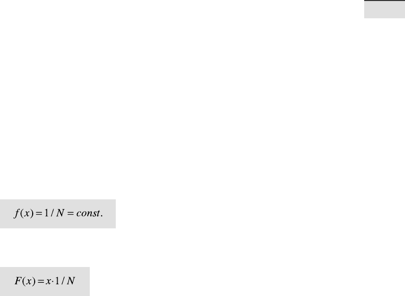
A uniform or rectangular distribution is a distribution that has a constant
probability (Fig. 3.4). e corresponding probability density function is
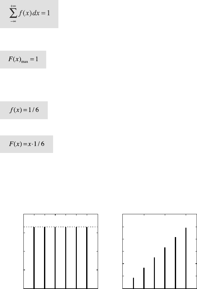
where the random variable x has any of N possible values. e cumulative
distribution function is
e probability density function is normalized to unity
52 3 UNIVARIATE STATISTICS
Fig. 3.4 a Probability density function f(x) and b cumulative distribution function F(x)
of a uniform distribution with N=6. e 6 discrete values of the variable x have the same
probability of 1/6.
123456
0
0.05
0.1
0.15
f(x)=1/6
0
1
1.2
0123456
0.2
0.2
0.4
0.8
0.6
xx
f(x)
F(x)
Cumulative Distribution
Function
Probability Density
Function
ab
i. e., the sum of all probabilities is one. e maximum value of the cumula-
tive distribution function is therefore one.
An example is a rolling die with N=6 faces. A discrete variable such as the
faces of a die can only take a countable number of values x. e probability
for each face is 1/6. e probability density function of this distribution is
e corresponding cumulative distribution function is
where x takes only discrete values, x=1,2,…,6.
3.4 THEORETICAL DISTRIBUTIONS 53
3 UNIVARIATE STATISTICS
Fig. 3.5 Probability density function f(x) of a binomial distribution, which gives the
probability p of x successes out of N=6 trials, with probability a p=0.1 and b p=0.3 of
success in any given trial.
012345
0
0123456
6
0.2
0.3
0.4
0.5
0.6
0.7
0.8
0.1
0
0.2
0.3
0.4
0.5
0.6
0.7
0.8
0.1
xx
f(x)
f(x)
Probability Density
Function
Probability Density
Function
p=0.1 p=0.3
ab
Binomial or Bernoulli Distribution
A binomial or Bernoulli distribution, named a er the Swiss scientist Jakob
Bernoulli (1654–1705), gives the discrete probability of x successes out of
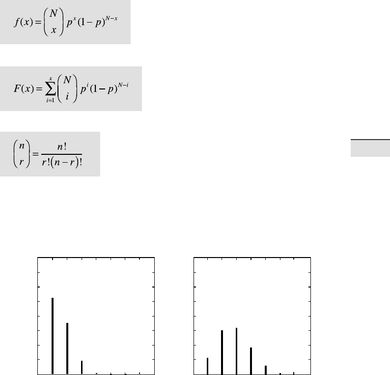
Ntrials, with a probability p of success in any given trial (Fig. 3.5). e prob-
ability density function of a binomial distribution is
e cumulative distribution function is
where
54 3 UNIVARIATE STATISTICS
λ=0.5 λ=2
0123456 0123456
0
0.2
0.3
0.4
0.5
0.6
0.7
0.8
0.1
0
0.2
0.3
0.4
0.5
0.6
0.7
0.8
0.1
xx
f(x)
f(x)
Probability Density
Function
Probability Density
Function
ab
Fig. 3.6 Probability density function f(x) of a Poisson distribution with di erent values
for λ. a λ=0.5 and b λ=2.
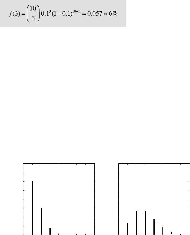
e binomial distribution has two parameters N and p. An example for the
application of this distribution is to determine the likely outcome of drilling
for oil. Let us assume that the probability of drilling success is 0.1 or 10 %. e
probability of x=3 successful wells out of a total number of N=10 wells is
e probability of exactly 3 successful wells out of 10 trials is therefore 6 %
in this example.
Poisson Distribution
When the number of trials is N →∞ and the success probability is p → 0,
the binomial distribution approaches a Poisson distribution with a single
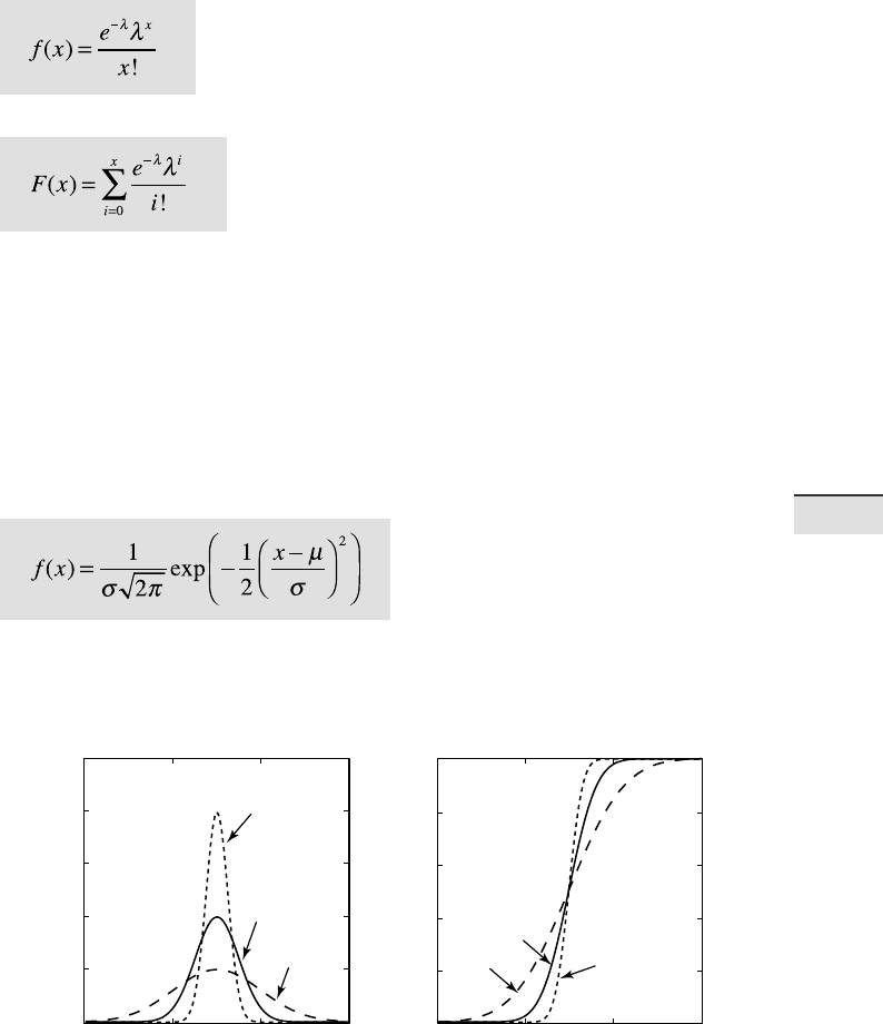
parameter λ=Np (Fig. 3.6) (Poisson 1837). is works well for N > 100 and
p < 0.05 or 5 %. We therefore use the Poisson distribution for processes char-
acterized by extremely low occurrence, e. g., earthquakes, volcanic erup-
tions, storms and oods. e probability density function is
3.4 THEORETICAL DISTRIBUTIONS 55
3 UNIVARIATE STATISTICS
σ =0.5
σ =1.0
σ =2.0
σ =0.5
σ =1.0
σ =2.0
0.2
0.4
0.6
0.8
0246
0.2
0.4
0.6
0.8
11
00
0246
xx
f(x)
F(x)
Probability Density
Function
Cumulative Distribution
Function
ab
Fig. 3.7 a Probability density function f(x) and b cumulative distribution function F(x)
of a Gaussian or normal distribution with a mean μ=3 and various values for standard
deviation σ.
and the cumulative distribution function is
e single parameter λ describes both the mean and the variance of this
distribution.
Normal or Gaussian Distribution
When p=0.5 (symmetric, no skew) and N→∞ , the binomial distribution
approaches a normal or Gaussian distribution de ned by the mean μ and
standard deviation σ (Fig. 3.7). e probability density function of a normal
distribution is
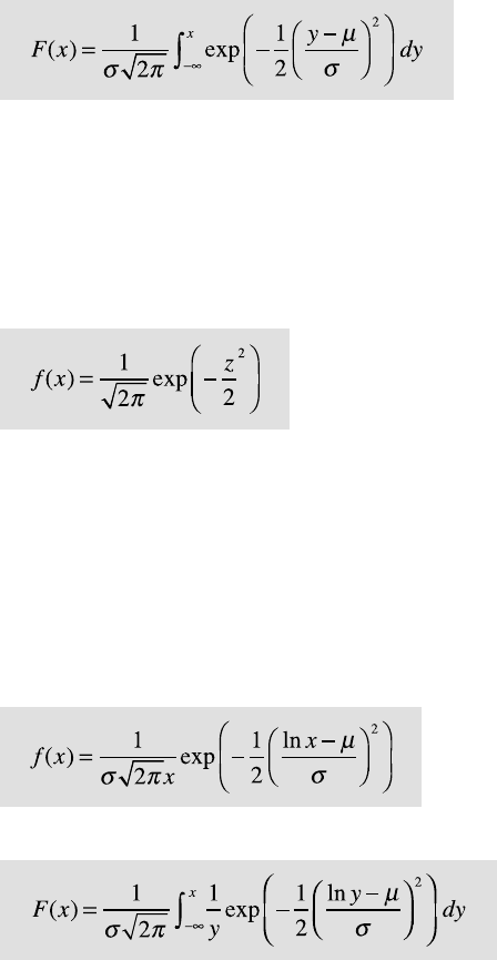
56 3 UNIVARIATE STATISTICS
and the cumulative distribution function is
e normal distribution is therefore used when the mean is both the most
frequent and the most likely value. e probability of deviations is equal in
either direction and decreases with increasing distance from the mean.
e standard normal distribution is a special member of the normal
distribution family that has a mean of zero and a standard deviation of one.
We can transform the equation for a normal distribution by substituting
z=(x–μ)/σ. e probability density function of this distribution is
is de nition of the normal distribution is o en called the z distribution.
Logarithmic Normal or Log-Normal Distribution
e logarithmic normal or log-normal distribution is used when the data
have a lower limit, e. g., mean-annual precipitation or the frequency of
earthquakes (Fig. 3.8). In such cases, distributions are usually characterized
by signi cant skewness, which is best described by a logarithmic normal
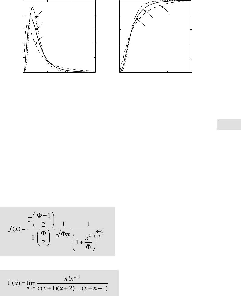
distribution. e probability density function of this distribution is
and the cumulative distribution function is
where x>0. e distribution can be described by two parameters: the mean
μ and the standard deviation σ. e formulas for the mean and the standard
deviation, however, are di erent from the ones used for normal distributions.
In practice, the values of x are logarithmized, the mean and the standard
deviation are computed using the formulas for a normal distribution, and
the empirical distribution is then compared with a normal distribution.
3.4 THEORETICAL DISTRIBUTIONS 57
3 UNIVARIATE STATISTICS
σ=0.5
σ=0.65
σ=1.0
σ=0.5
σ=0.65
σ=1.0
0.2
0.4
0.6
0.8
0246
0.2
0.4
0.6
0.8
11
00
0246
xx
f(x)
F(x)
Probability Density
Function
Cumulative Distribution
Function
ab
Fig. 3.8 a Probability density function f(x) and b cumulative distribution function F(x) of a
logarithmic normal distribution with a mean μ=0 and with various values for σ.
Student’s t Distribution
e Student’s t distribution was rst introduced by William Gosset (1876–
1937) who needed a distribution for small samples (Fig. 3.9). Gosset was
an employee of the Irish Guinness Brewery and was not allowed to publish
research results. For that reason he published his t distribution under the
pseudonym Student (Student 1908). e probability density function is
where Γ is the Gamma function
which can be written as
