Tietenberg Tom, Lewis Lynne. Environmental & Natural Resource Economics
Подождите немного. Документ загружается.

101Further Reading
of essays by some of the chief practitioners in the field evaluating both the legal frame-
work for damage assessment and the validity and reliability of the methods currently
being used. Robert Cameron, Mitchell, and Richard T. Carson. Using Surveys to Value
Public Goods: The Contingent Valuation Method (Washington, DC: Resources for the
Future, 1989). A comprehensive examination of contingent valuation research with brief
summaries of representative studies.
Lewis, Lynne Y., Curtis Bohlen, and Sarah Wilson. “Dams, Dam Removal and River
Restoration: A Hedonic Analysis,” Contemporary Economic Policy Vol. 26, No. 2 (2008):
175–186.
Additional References and Historically Significant References are available on this book’s
Companion Website: http://www.pearsonhighered.com/tietenberg/

102
5
5
Dynamic Efficiency and
Sustainable Development
We usually see only the things we are looking for—so much so that we
sometimes see them where they are not
—Eric Hoffer, The Passionate State of Mind (1993)
Introduction
In previous chapters, we have developed two specific means for identifying
environmental problems. The first, static efficiency, allows us to evaluate those
circumstances where time is not a crucial aspect of the allocation problem. Typical
examples might include allocating resources such as water or solar energy where
next year’s flow is independent of this year’s choices. The second, more
complicated criterion, dynamic efficiency, is suitable for those circumstances
where time is a crucial aspect. One typical example might include the combustion
of depletable resources such as oil, since supplies used now are unavailable for
future generations.
After defining these criteria and showing how they could be operationally
invoked, we demonstrated how helpful they can be. They are useful not only
in identifying environmental problems and ferreting out their behavioral sources,
but also in providing a basis for identifying types of remedies. These criteria even
help design the various policy instruments that can be used to restore some sense
of balance.
But the fact that these are powerful and useful tools in the quest for a sense of
harmony between the economy and the environment does not imply that they are
the only criteria in which we should be interested. In a general sense, the efficiency
criteria are designed to prevent wasteful use of environmental and natural
resources. That is a desirable attribute, but it is not the only possible desirable
attribute. We might care, for example, not only about the value of the environment
(the size of the pie), but also how this value is shared (the size of each piece to all
recipients). In other words, fairness or justice concerns should accompany
efficiency considerations.
In this chapter, we investigate one particular fairness concern—the treatment of
future generations. We begin by considering a specific, ethically challenging
situation—the allocation of a depletable resource over time. Using a numerical
103A Two-Period Model
example, we shall trace out the temporal allocation of a depletable resource using
the dynamic efficiency criterion and show how this allocation is affected by changes
in the discount rate. To lay the groundwork for our evaluation of fairness, we then
turn to the task of defining what we mean by intertemporal fairness. Finally, we
consider not only how this theoretical definition can be made operationally
measurable, but also how it relates to dynamic efficiency. To what degree is
dynamic efficiency compatible with intergenerational fairness?
A Two-Period Model
Dynamic efficiency balances present and future uses of a depletable resource by
maximizing the present value of the net benefits derived from its use. This implies a
particular allocation of the resource across time. We can investigate the properties
of this allocation and the influence of such key parameters as the discount rate with
the aid of a simple numerical example. We begin with the simplest of models—
deriving the dynamic efficient allocation across two time periods. In subsequent
chapters, we show how these conclusions generalize to longer time periods and to
more complicated situations.
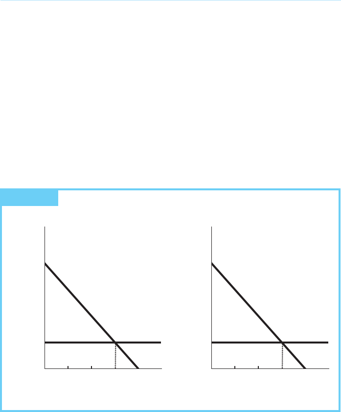
Assume that we have a fixed supply of a depletable resource to allocate between
two periods. Assume further that the demand function is constant in the two
periods, the marginal willingness to pay is given by the formula P ⫽ 8 ⫺ 0.4q, and
marginal cost is constant at $2 per unit (see Figure 5.1). Note that if the total supply
was 30 or greater, and we were concerned only with these two periods, an efficient
allocation would produce 15 units in each period, regardless of the discount rate.
Price
(dollars
per unit)
Quantity
(units)
0
(b)
5
2
8
10 15 20
M
C
Price
(dollars
per unit)
Quantity
(units)
0
(a)
5
2
8
10 15 20
MC
FIGURE 5.1 The Allocation of an Abundant Depletable Resource: (a) Period 1
and (b) Period 2

104 Chapter 5 Dynamic Efficiency and Sustainable Development
Thirty units would be sufficient to cover the demand in both periods; the
consumption in Period 1 does not reduce the consumption in Period 2. In this
case the static efficiency criterion is sufficient because the allocations are not
interdependent.
Examine, however, what happens when the available supply is less than 30.
Suppose it equals 20. How do we determine the efficient allocation? According to
the dynamic efficiency criterion, the efficient allocation is the one that maximizes
the present value of the net benefit. The present value of the net benefit for both
periods is simply the sum of the present values in each of the two periods. To take a
concrete example, consider the present value of a particular allocation: 15 units in
the first period and 5 in the second. How would we compute the present value of
that allocation?
The present value in the first period would be that portion of the geometric
area under the demand curve that is over the supply curve—$45.00.
1
The present
value in the second period is that portion of the area under the demand curve that
is over the supply curve from the origin to the five units produced multiplied by
1/(1 ⫹ r). If we use r ⫽ 0.10, then the present value of the net benefit received in
the second period is $22.73,
2
and the present value of the net benefits for the two
years is $67.73.
Having learned how to find the present value of net benefits for any
allocation, how does one find the allocation that maximizes present value? One
way, with the aid of a computer, is to try all possible combinations of q
1
and q
2
that sum to 20. The one yielding the maximum present value of net benefits can
then be selected. That is tedious and, for those who have the requisite
mathematics, unnecessary.
The dynamically efficient allocation of this resource has to satisfy the condition
that the present value of the marginal net benefit from the last unit in Period 1
equals the present value of the marginal net benefit in Period 2 (see appendix at the
end of this chapter). Even without mathematics, this principle is easy to
understand, as can be demonstrated with the use of a simple graphical
representation of the two-period allocation problem.
Figure 5.2 depicts the present value of the marginal net benefit for each of the
two periods. The net benefit curve for Period 1 is to be read from left to right.
The net benefit curve intersects the vertical axis at $6; demand would be zero at $8
and the marginal cost is $2, so the difference (marginal net benefit) is $6. The
marginal net benefit for the first period goes to zero at 15 units because, at that
quantity, the willingness to pay for that unit exactly equals its cost.
The only challenging aspect of drawing the graph involves constructing the
curve for the present value of net benefits in Period 2. Two aspects are worth
noting. First, the zero axis for the Period 2 net benefits is on the right, rather
than the left, side. Therefore, increases in Period 2 are recorded from right to
left. This way, all points along the horizontal axis yields a total of 20 units
1
The height of the triangle is $6 [$8–$2] and the base is 15 units. The area is therefore (1/2)($6)(15) ⫽ $45.
2
The undiscounted net benefit is $25. The calculation is (6 ⫺ 2) ⫻ 5 ⫹ 1/2(8 ⫺ 6) ⫻ 5 ⫽ $25.
The discounted net benefit is therefore 25/1.10 ⫽ 22.73.

105A Two-Period Model
Quantity in
Period 2
0 1 2 3 4 5 6 7 8 9 10111213141516171819 20
19 18 17 16 15 14 13 12 11 10 9 8 7 6 5 4 3 2 1 0
1
2
3
4
5
5.45
6
Marginal Net
Benefits in
Period 1
(dollars
per unit)
Marginal Net
Benefits in
Period 2
(dollars
per unit)
Present Value of Marginal Net
Benefits in Period 2
Present Value of Marginal Net
Benefits in Period 1
1
2
3
4
5
6
20
Quantity in
Period 1
FIGURE 5.2 The Dynamically Efficient Allocation
allocated between the two periods. Any point on that axis picks a unique
allocation between the two periods.
3
Second, the present value of the marginal benefit curve for Period 2 intersects
the vertical axis at a different point than does the comparable curve in Period 1.
(Why?) This intersection is lower because the marginal benefits in the second
period need to be discounted (multiplied by 1/(1 ⫹ r)) to convert them into present
value form since they occur one year later. Thus, with the 10 percent discount rate
we are using, the marginal net benefit is $6 and the present value is $6/1.10 ⫽ $5.45.
Note that larger discount rates would rotate the Period 2 marginal benefit curve
around the point of zero net benefit (q
1
⫽ 5, q
2
⫽ 15) toward the right-hand axis.
We shall use this fact in a moment.
The efficient allocation is now readily identifiable as the point where the two
curves representing present value of marginal net benefits cross. The total present
value of net benefits is then the area under the marginal net benefit curve for Period
1 up to the efficient allocation, plus the area under the present value of the marginal
net benefit curve for Period 2 from the right-hand axis up to its efficient allocation.
Because we have an efficient allocation, the sum of these two areas is maximized.
4
3
Note that the sum of the two allocations in Figure 5.2 is always 20. The left-hand axis represents an
allocation of all 20 units to Period 2, and the right-hand axis represents an allocation entirely to
Period 1.
4
Demonstrate that this point is the maximum by first allocating slightly more to Period 2 (and therefore
less to Period 1) and showing that the total area decreases. Conclude by allocating slightly less to Period
2 and showing that, in this case as well, total area declines.
106 Chapter 5 Dynamic Efficiency and Sustainable Development
Since we have developed our efficiency criteria independent of an institutional
context, these criteria are equally appropriate for evaluating resource allocations
generated by markets, government rationing, or even the whims of a dictator.
While any efficient allocation method must take scarcity into account, the details of
precisely how that is done depend on the context.
Intertemporal scarcity imposes an opportunity cost that we henceforth refer to
as the marginal user cost. When resources are scarce, greater current use diminishes
future opportunities. The marginal user cost is the present value of these forgone
opportunities at the margin. To be more specific, uses of those resources, which
would have been appropriate in the absence of scarcity, may no longer be
appropriate once scarcity is present. Using large quantities of water to keep lawns
lush and green may be wholly appropriate for an area with sufficiently large
replenishable water supplies, but quite inappropriate when it denies drinking water
to future generations. Failure to take the higher scarcity value of water into account
in the present would lead to inefficiency due to the additional cost resulting from
the increased scarcity imposed on the future. This additional marginal value
created by scarcity is the marginal user cost.
We can illustrate this concept by returning to our numerical example. With 30 or
more units, each period would be allocated 15, the resource would not be scarce,
and the marginal user cost would be zero.
With 20 units, however, scarcity emerges. No longer can 15 units be allocated to
each period; each period will have to be allocated less than would be the case
without scarcity. Due to this scarcity the marginal user cost for this case is not zero.
As can be seen from Figure 5.2, the present value of the marginal user cost, the
additional value created by scarcity, is graphically represented by the vertical
distance between the quantity axis and the intersection of the two present-value
curves. It is identical to the present value of the marginal net benefit in each of the
periods. This value can either be read off the graph or determined more precisely,
as demonstrated in the chapter appendix, to be $1.905.
We can make this concept even more concrete by considering its use in a
market context. An efficient market would have to consider not only the
marginal cost of extraction for this resource but also the marginal user cost.
Whereas in the absence of scarcity, the price would equal only the marginal cost
of extraction, with scarcity, the price would equal the sum of marginal extraction
cost and marginal user cost.
To see this, solve for the prices that would prevail in an efficient market facing
scarcity over time. Inserting the efficient quantities (10.238 and 9.762, respectively)
into the willingness-to-pay function (P ⫽ 8 ⫺ 0.4q) yields P
1
⫽ 3.905 and P
2
⫽ 4.095.
The corresponding supply-and-demand diagrams are given in Figure 5.3.
Compare Figure 5.3 with Figure 5.1 to see the impact of scarcity on price.
Note that in the absence of scarcity, marginal user cost is zero.
In an efficient market, the marginal user cost for each period is the difference
between the price and the marginal cost of extraction. Notice that it takes the value
$1.905 in the first period and $2.095 in the second. In both the periods, the present
value of the marginal user cost is $1.905. In the second period, the actual marginal
user cost is $1.905(l ⫹ r). Since r ⫽ 0.10 in this example, the marginal user cost for

107Defining Intertemporal Fairness
Price
(dollars
per unit)
Quantity
(units)
0
(b)
2.000
4.095
8
9.762 20
MC
D
P
Price
(dollars
per unit)
Quantity
(units)
0
(a)
2.000
3.905
8
10.238 20
MC
D
P
FIGURE 5.3 The Efficient Market Allocation of a Depletable Resource:
The Constant-Marginal-Cost Case: (a) Period 1 and (b) Period 2
the second period is $2.095.
5
Thus, while the present value of marginal user cost
is equal in both periods, the actual marginal user cost rises over time.
Both the size of the marginal user cost and the allocation of the resource
between the two periods is affected by the discount rate. In Figure 5.2, because of
discounting, the efficient allocation allocates somewhat more to Period 1 than to
Period 2. A discount rate larger than 0.10 would be incorporated in this diagram by
rotating the Period 2 curve an appropriate amount toward the right-hand axis,
holding fixed the point at which it intersects the horizontal axis. (Can you see why?)
The larger the discount rate, the greater the amount of rotation required.
The amount allocated to the second period would be necessarily smaller with
larger discount rates. The general conclusion, which holds for all models we
consider, is that higher discount rates tend to skew resource extraction toward the
present because they give the future less weight in balancing the relative value of
present and future resource use. The choice of what discount rate to use, then,
becomes a very important consideration for decision makers.
Defining Intertemporal Fairness
While no generally accepted standards of fairness or justice exist, some have more
prominent support than others. One such standard concerns the treatment of
future generations. What legacy should earlier generations leave to later ones?
5
You can verify this by taking the present value of $2.095 and showing it to be equal to $1.905.

108 Chapter 5 Dynamic Efficiency and Sustainable Development
This is a particularly difficult issue because, in contrast to other groups for which
we may want to ensure fair treatment, future generations cannot articulate their
wishes, much less negotiate with current generations. (“We’ll take your radioactive
wastes, if you leave us plentiful supplies of titanium.”)
One starting point for intergenerational equity is provided by philosopher John
Rawls in his monumental work, A Theory of Justice. Rawls suggests one way to
derive general principles of justice is to place, hypothetically, all people into an
original position behind a “veil of ignorance.” This veil of ignorance would prevent
them from knowing their eventual position in society. Once behind this veil, people
would decide on rules to govern the society that they would, after the decision, be
forced to inhabit.
In our context, this approach would suggest a hypothetical meeting of all
members of present and future generations to decide on rules for allocating
resources among generations. Because these members are prevented by the veil of
ignorance from knowing the generation to which they will belong, they will not be
excessively conservationist (lest they turn out to be a member of an earlier
generation) or excessively exploitative (lest they become a member of a later
generation).
What kind of rule would emerge from such a meeting? One possibility is the
sustainability criterion. The sustainability criterion suggests that, at a minimum,
future generations should be left no worse off than current generations. Allocations
that impoverish future generations, in order to enrich current generations, are,
according to this criterion, patently unfair.
In essence, the sustainability criterion suggests that earlier generations are at
liberty to use resources that would thereby be denied to future generations as long
as the well-being of future generations remains just as high as that of all previous
generations. On the other hand, diverting resources from future use would violate
the sustainability criterion if it reduced the well-being of future generations below
the level enjoyed by preceding generations.
One of the implications of this definition of sustainability is that it is possible for
the current generation to use resources (even depletable resources) as long as
the interests of future generations could be protected. Do our institutions provide
adequate protection for future generations? We begin with examining the
conditions under which efficient allocations satisfy the sustainability criterion.
Are all efficient allocations sustainable?
Are Efficient Allocations Fair?
In the numerical example we have constructed, it certainly does not appear that the
efficient allocation satisfies the sustainable criterion. In the two-period example,
more resources are allocated to the first period than to the second. Therefore, net
benefits in the second period are lower than in the first. Sustainability does not
allow earlier generations to profit at the expense of later generations, and this
example certainly appears to be a case where that is happening.

109Are Efficient Allocations Fair?
Yet choosing this particular extraction path does not prevent those in the first
period from saving some of the net benefits for those in the second period. If the
allocation is dynamically efficient, it will always be possible to set aside sufficient
net benefits accrued in the first period for those in the second period, so that those
in the second period will be at least as well off as they would have been with any
other extraction profile.
We can illustrate this point with a numerical example that compares a dynamic
efficient allocation with sharing to an allocation where resources are committed
equally to each generation. Suppose, for example, you believe that setting aside half
(10 units) of the available resources for each period would be a better allocation
than the dynamic efficient allocation. The net benefits to each period from this
alternative scheme would be $40. Can you see why?
Now let’s compare this to an allocation of net benefits that could be achieved
with the dynamic efficient allocation. If the dynamic efficient allocation is to satisfy
the sustainability criterion, we must be able to show that it can produce an outcome
such that each generation would be at least as well off as it would be with the equal
allocation. Can that be demonstrated?
In the dynamic efficient allocation, the net benefits to the first period were
40.466, while those for the second period were 39.512.
6
Clearly, if no sharing
between the periods took place, this example would violate the sustainability
criterion; the second generation is worse off.
But suppose the first generation was willing to share some of the net benefits
from the extracted resources with the second generation. If the first generation
keeps net benefits of $40 (thereby making it just as well off as if equal amounts
were extracted in each period) and saves the extra $0.466 (the $40.466 net
benefits earned during the first period in the dynamic efficient allocation minus
the $40 reserved for itself) at 10 percent interest for those in the next period,
this savings would grow to $0.513 by the second period [0.466(1.10)]. Add this
to the net benefits received directly from the dynamic efficient allocation
($39.512), and the second generation would receive $40.025. Those in the
second period would be better off by accepting the dynamic efficient allocation
with sharing than they would if they demanded that resources be allocated
equally between the two periods.
This example demonstrates that although dynamic efficient allocations do not
automatically satisfy sustainability criteria, they could be compatible with sustain-
ability, even in an economy relying heavily on depletable resources. The possibility
that the second period can be better off is not a guarantee; the required degree of
sharing must take place. Example 5.1 points out that this sharing does sometimes
take place, although, as we shall see, such sharing is more likely to be the exception
rather than the norm. In subsequent chapters, we shall examine both the conditions
under which we could expect the appropriate degree of sharing to take place and
the conditions under which it would not.
6
The supporting calculations are (1.905)(10.238) + 0.5(4.095)(10.238) for the first period and
(2.095)(9.762) + 0.5(3.905)(9.762) for the second period.

110 Chapter 5 Dynamic Efficiency and Sustainable Development
The Alaska Permanent Fund
One interesting example of an intergenerational sharing mechanism currently
exists in the State of Alaska. Extraction from Alaska’s oil fields generates
significant income, but it also depreciates one of the state’s main environmental
assets. To protect the interests of future generations as the Alaskan pipeline
construction neared completion in 1976, Alaska voters approved a constitutional
amendment that authorized the establishment of a dedicated fund: the Alaska
Permanent Fund. This fund was designed to capture a portion of the rents
received from the sale of the state’s oil to share with future generations.
The amendment requires:
At least 25 percent of all mineral lease rentals, royalties, royalty sales
proceeds, federal mineral revenue-sharing payments and bonuses received by
the state be placed in a permanent fund, the principal of which may only be
used for income-producing investments.
The principal of this fund cannot be used to cover current expenses without a
majority vote of Alaskans.
The fund is fully invested in capital markets and diversified among various
asset classes. It generates income from interest on bonds, stock dividends, real
estate rents, and capital gains from the sale of assets.
7
To date, the legislature has
used some of these annual earnings to provide dividends to every eligible Alaska
resident, while using the rest to increase the size of the principal, thereby
assuring that it is not eroded by inflation. The 2010 dividend was $1,281.
Although this fund does preserve some of the revenue for future generations,
two characteristics are worth noting. First, the principal could be used for current
expenditures if a majority of current voters agreed. To date, that has not
happened, but it has been discussed. Second, only 25 percent of the oil revenue
is placed in the fund; assuming that revenue reflects scarcity rent, full
sustainability would require dedicating 100 percent of it to the fund. Because the
current generation not only gets its share of the income from the permanent fund,
but also receives 75 percent of the proceeds from current oil sales, this sharing
arrangement falls short of that prescribed by the Hartwick Rule.
Source
: The Alaska Permanent Fund Web site: http://www.pfd.state.ak.us/
EXAMPLE
5.1
Applying the Sustainability Criterion
One of the difficulties in assessing the fairness of intertemporal allocations using
this version of the sustainability criterion is that it is so difficult to apply.
Discovering whether the well-being of future generations is lower than that of
current generations requires us not only to know something about the allocation of
7
The fund is managed by the Alaska Permanent Fund Corporation. http://www.apfc.org/
home/Content/home/index.cfm