Teodorescu P.P. Mechanical Systems, Classical Models Volume I: Particle Mechanics

Подождите немного. Документ загружается.

MECHANICAL SYSTEMS, CLASSICAL MODELS

100

{}

{

}

≡VRM.

(2.2.24'')

Because the moment of a bound vector with respect to a pole holds also for a sliding

vector, the definition given above is valid as well for a system of sliding vectors. The

components of the resultant and of the resultant moment can be written in the form

∑

=∈

∑

()

Ox jkl il

MxV

, 1, 2, 3j

(2.2.24''')

Let

{}

, , 1,2,..., , 1,2,...,

injm

′′

+= = =

VV VV be the sum of two systems

of vectors, where

{}

{

}

, 1,2,...,

′′

≡=VV is another system of bound or sliding

vectors. As well, let be a scalar

λ and a system of vectors

{

}

V ; the product of λ by

{}

V is of the form

{}

{

}

,1,2,...,

inλλλ

≡

≡=VVV . The two operations

mentioned above have all the properties which are put in evidence in Chap. 1, Subsec.

1.1.2 concerning the addition of vectors or the product of a scalar by a vector. In

particular, we can take

1λ

− , which leads to the operation

{}

′

−

VV. The

definition of the torsor of a system of vectors yields the basic properties:

{}

(

)

{}

{

}

OOO

′′

τ+=τ+τ

VV V V;

ii)

{}

(

)

{}

λλτ=τVV.

Hence, the torsor is a linear operator. We notice also that the torsor is invariant with

respect to the group of elementary operations of equivalence or with respect to the

enlarged group of these operations, as we have to do with systems of bound or sliding

vectors, respectively.

If a system of vectors

{}

V is equivalent to zero, then its torsor at an arbitrary pole

O is equal to zero

{

}

=V0,

(2.2.25)

which is equivalent to

R0,

M0.

(2.2.25')

Indeed, supposing that we have to do with a system of bound vectors, the resultant at

each point of the system must vanish, the affirmation being thus justified. A system of

sliding vectors is reduced to a system of two sliding vectors, which verify a relation of

the form (1.1.11), the vectors having the same support; we are thus led to a relation of

the form (2.2.6) too, hence the affirmation is justified also in this case.

Let be now a system of sliding vectors for which the torsor vanishes. We can reduce

this system to a system of two sliding vectors

{}

{

}

≡

UUU; but the torsor is an

invariant, so that it vanishes also for this system of sliding vectors. Because the resultant

of the system

{}

U is equal to zero, we can state that the vectors

and

have the

same modulus, but opposite directions; their supports can be parallel (

+=UU 0, as

Mechanics of the systems of forces

101

free vectors). The resultant moment of the system

{

}

U also vanishes, so that the two

supports must coincide. Indeed the condition

1122

+× =rU rU 0 leads to the

condition

()

21 2 12 2

PP−×= ×=





rr U U 0, the above affirmation being thus justified

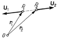
(Fig.2.13); by sliding along the common support, it is seen that the system

{}

U is

equivalent to zero. Hence, a system of sliding vectors is equivalent to zero, and we write

this in the form (2.2.19), if and only if its torsor vanishes; in the case of a system of

bound vectors, the condition (2.2.25) is only necessary. Taking into account (2.2.24'''),

this condition leads to six equations of projection on the three axes of co-ordinates.

Figure 2.13. Torsor of a system of two sliding vectors equivalent to zero.

Let

{}

V and

{}

′

V be two equivalent systems of vectors, so that one can write the

relation (2.2.18); it results

{}

{

}

{}

′

−

∼VV 0, and further

{}

(

)

′

−=VV 0.

Noting that the torsor is a linear operator, we state that two systems of sliding vectors

are equivalent, and we write the relation (2.2.18), if and only if their torsors with

respect to the same pole are equal

{}

{

}

′

=τVV;

(2.2.26)

in the case of systems of bound vectors, the condition (2.2.26) is only necessary.

The resultant

R of the system of vectors

{

}

V is invariant by a change of pole O .

In what concerns the resultant moment, by passing to a pole

′

, we obtain

(

)

11 11

nn nn

ii i i i ii

ii ii

OP OO OP OO OP

′

== ==

′′ ′

=×= +×=×+×

∑∑ ∑∑



  



 

MV VVV

so that

′

+×





MM R

(2.2.27)

{} {}

{

}

′

τ=τ+ ×





VV0R

(2.2.27')

a relation of the same form as the relation (2.2.15); we obtain thus the variation of the

resultant moment, hence also of the torsor of a system of vectors, by a change of the

pole with respect to which this torsor is calculated. The torsor of a system of vectors is

invariant by a change of pole

O if this pole moves along an axis parallel to the resultant

R or if this one vanishes. Hence, if the torsor of a system of vectors equivalent to zero

MECHANICAL SYSTEMS, CLASSICAL MODELS

102

vanishes at a point (

{}

τ=V0

), then it is equal to zero at any other point

(

{}

′

τ=V0); otherwise, the equivalence to zero of a system of sliding vectors would

depend on the pole with respect to which the torsor is calculated.

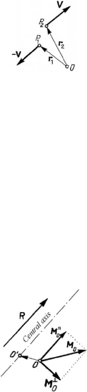
Figure 2.14. Couple of two sliding vectors.

A system of sliding vectors for which

R0 and

≠

M0 is reducible to a system

formed by two sliding vectors having the same modulus, parallel supports and opposite

directions (Fig.2.14). Such a system is called a couple, and its torsor – as we have seen

– is invariant by a change of pole.

A scalar product of the relation (2.2.27) by

R leads to

′

⋅

=⋅RM RM,

(2.2.28)

observing that we obtain also a mixed product equal to zero; this quantity is called the

torsor’s scalar and is invariant by a change of pole. Let be

OOO

⊥

+MMM

(2.2.29)

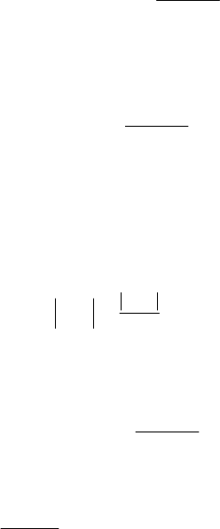
where we have decomposed the moment

M into two components: a component

parallel and a component normal to the resultant

R , respectively (Fig.2.15); in this

case, the relation (2.2.28) is equivalent to

Figure 2.15. Central axis of a system of sliding vectors.

′

⋅

=⋅RM RM

(2.2.28')

because

⊥

⋅=RM . Hence, the component of the resultant moment along the

resultant

is also an invariant by a change of pole

′

(2.2.28'')

Mechanics of the systems of forces

103

In this case, the relation (2.2.27) leads to

⊥⊥

′

+×





MM R

(2.2.27'')

We put the problem to find a pole with respect to which the torsor of a system of

vectors has the simplest form possible (the minimal form). Because

R and

are

invariants, the only quantity varying in modulus, together with the pole

O , is

⊥

M ; we

will try to find a pole with respect to which this component of the resultant moment

vanishes. If the pole

′

has this property, then the relation (2.2.27'') allows us to write

the condition

⊥

′

×=





MR0

We obtain thus a vector equation of the form (2.1.54); using the solution (2.1.54'), we

may write

⊥

′





where

λ is an arbitrary scalar; we notice that this solution may be written also in the

form

′





(2.2.30)

because

=RM 0

. We obtain thus an axis parallel to the resultant R ; the resultant

moments with respect to its points have only the invariant component

. We say, in

this case, that the torsor takes its minimal form; the respective axis is called the central

axis of the system of vectors (Fig.2.15). For

0λ

, we obtain OO

′

⊥





, with

⊥

′





(2.2.30')

A vector product of the relation (2.2.30) at left by

R allows us to eliminate λ , and we

obtain

′

×=×





(2.2.31)

The formula of the triple vector product leads to

⋅

′

−×





RM R

(2.2.31')

Taking the pole

O as origin of the co-ordinate axes and denoting the co-ordinates of the

point

′

by ,1,2,3

xi= , we can write

MECHANICAL SYSTEMS, CLASSICAL MODELS

104

()()

23 32 31 13

Ox Ox

MxRxR MxRxR

−+ = −+

()()

3123

12 21 1 2 3

Ox Ox Ox Ox

MxRxR RMRMRM

=−+= ++;

(2.2.31'')

these equations represent two planes, the intersection of which is the central axis.

As we have seen, the torsor operator characterizes a system of sliding vectors; thus,

taking into account the form of the torsor, we can distinguish several cases of reduction

of such a system of vectors to simpler systems, i.e.:

=R0 and

M0, then we obtain a system of sliding vectors equivalent

to zero.

ii)

≠R0 and

M0, then the system of sliding vectors is equivalent to a

resultant having as support the central axis; indeed, because

⊥

=M0, the pole

belongs to this axis, so that the affirmation is justified.

iii)

=R0 and

≠

M0, then the system of sliding vectors is equivalent to a

couple.

iv)

≠R0 and

≠

M0, then we distinguish two subcases:

iv')

⋅=RM , then the system of sliding vectors is equivalent to a

resultant, the support of which is the central axis; indeed, in this case

=M0

. It is a difference between the cases ii) and iv'), because – in the

latter case – the pole

O does not belong obligatory to the central axis.

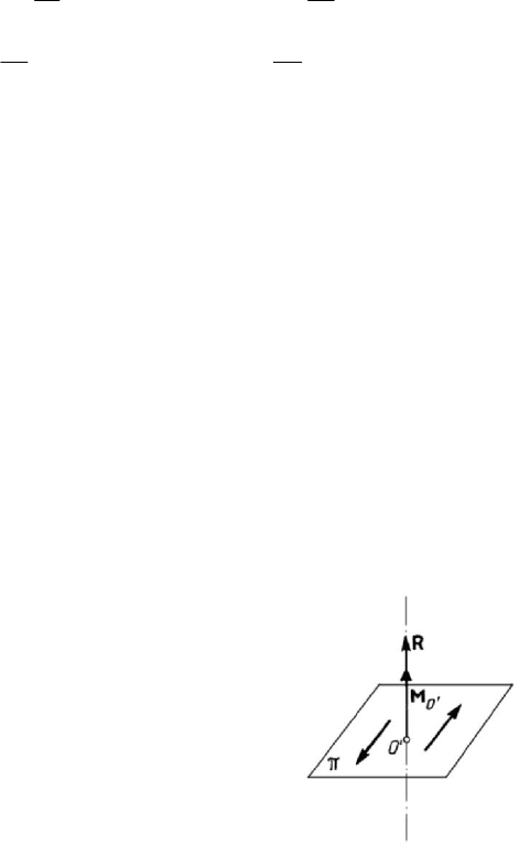
Figure 2.16. Dynam of a system of sliding vectors for which the

torsor’s scalar does not vanish.

iv'')

If the torsor’s scalar

⋅

≠RM

, that is in the general case, then the

system of sliding vectors is equivalent to a dynam (or a screw); the

support of the resultant

R is the central axis, while the resultant moment

leads to a couple of moment

′

(the point O

′

on the central axis),

acting in a plane

Π normal to this resultant (Fig.2.16).

2.2.6 Systems of coplanar forces

In the case of a system of coplanar forces

{}

{

}

, 1,2,...,

≡

=FF , modelled by

sliding vectors, the resultant is – obviously – contained in the considered plane

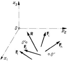
Mechanics of the systems of forces

105

(Fig.2.17). The moment

of the system of forces with respect to a pole

O Π∈

will

be a vector normal to the resultant

R ; hence, 0

⋅

=RM and we are in the case iv').

≠R0, then the system of coplanar forces modelled by sliding vectors is reduced to

a resultant along the central axis, contained in the considered plane. If the resultant

vanishes, then the system of forces reduces to a couple if

≠

(with respect to an

arbitrary point in the plane) or is equal to zero if

M0.

Figure 2.17. Systems of coplanar forces.

Supposing that this system of forces acts in the plane

Ox x , the conditions of

equivalence to zero are written in the form

0RR==,

(2.2.32)

In particular, a system of three non-parallel coplanar forces modelled by sliding

vectors, the resultant of which vanishes (

0RR

), is equivalent to zero if and

only if the three forces are concurrent (we use the condition

). But choosing

two poles

′

and O

′′

in the plane and writing the conditions

′

=+×=





MM R0

′′

+×=





MM R0

we state that a system of coplanar forces modelled by sliding vectors is equivalent to

zero if and only if the conditions

=M0,

′

M0,

′′

(2.2.33)

are fulfilled, the poles

O , O

′

and O

′

being non-collinear; these conditions lead to

three projection equations on the axis

Ox , which can be useful in applications. We

mention that, for the equivalence to zero of a system of coplanar forces modelled by

bound vectors, these conditions are only necessary.

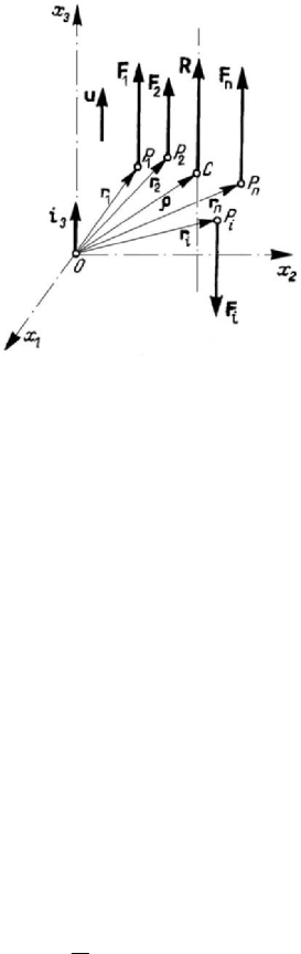
2.2.7 Systems of parallel forces

Let be a direction of unit vector

and a system of parallel forces

{}

, 1,2,...,

in≡=FF , modelled by sliding vectors and given by

MECHANICAL SYSTEMS, CLASSICAL MODELS

106

;

(2.2.34)

Figure 2.18. Systems of parallel forces.

these forces are applied at the points

P , of position vectors ,1,2,...,

r (Fig.2.18).

We notice that

represent the components of these forces along the given direction,

having

vers

=±Fu. The resultant of this system of forces will be

∑

RFu,

(2.2.35)

where we have used the notation

∑

(2.2.35')

The resultant moment with respect to the pole

O is written in the form

×=×

∑

MrFRρ ,

where we took into consideration the resultant (2.2.35), defining the vector

∑

rρ

(2.2.36)

and admitting that

0F ≠ . The position vector

determines a point C with respect to

which the resultant moment vanishes (

+×=





MM R0

); hence, the point C

belongs to the central axis, which is determined by the unit vector

u . The system of

parallel forces modelled by sliding vectors is reduced, in this case, to a resultant along

the central axis. We have

⋅

=RM and are in the case iv').

Mechanics of the systems of forces

107

0F =

, then =R0, and the system of forces modelled by sliding vectors is

reduced to a couple if

≠

M0 or is equivalent to zero if

M0. Supposing that the

forces of the system

{}

F are parallel to the axis

, i.e.,

(Fig.2.18), the

conditions of equivalence to zero are written in the form

0R = ,

Ox Ox

(2.2.37)

The above conditions are only necessary in the case of parallel forces modelled by

bound vectors.

The point

C is called the centre of the system of parallel forces modelled by sliding

vectors, through it passing the central axis of the respective system. One obtains the

same centre

C for the system

{

}

λ F , λ scalar. Let

{

}

{

}

, 1,2,...,

′

≡

=FF be

another system of parallel forces modelled by sliding vectors, the supports of which

pass through the same points, respectively, but have another direction, given by the unit

vector

′

u (

′′′

Fu), and which have the same components as the system of forces

{

}

F (that is , 1,2,...,

FFi n

′

); in fact, it is a rotation of the same angle of all the

supports. One obtains the same centre

C of the system of parallel forces, the central

axis having – obviously – the direction given by the new unit vector

′

u .

2.2.8 Other considerations concerning systems of forces

Let

{

}

, , 1,2,...,

≡

=FrF be a system of forces modelled by bound vectors,

where we put into evidence also the position vectors of the points of application; the

torsor of this system with respect to the pole

O is

{

}

{

}

τ=F RM ,

(2.2.38)

where the resultant and the resultant moment are given by

∑

RF,

∑

MrF.

(2.2.38')

We notice that, excepting the so-called forces, a mechanical system is acted upon by a

couple of forces (or a moment) too; we use also the generic denomination of charge

(load).

The considered system of forces

F corresponds rigorously to a discrete mechanical

system; we have seen in Chap. 1, Subsec. 1.1.11 that, in the case of a continuous

mechanical system, which has as support a domain

D , the load can be punctual, linear,

superficial or volumic, corresponding to the dimensions of the subdomain

D⊂D to

which it is transmitted.

The torsor (2.3.38), corresponding to a distributed load on a line

L , a surface S or a

volume

V , respectively will be given by

∫

Rp , d

∫

Rp , d

∫

Rf ,

(2.2.39)

s=×

∫

Mrp , d

S=×

∫

Mrp , d

V=×

∫

Mrf ,

(2.2.39')

MECHANICAL SYSTEMS, CLASSICAL MODELS

108

where

p and

are continuous functions, representing loads on a unit of line, of area or

of volume, respectively; these unit loads are vector quantities. Obviously, we may use

also the notation of mean unit load

mean

(2.2.40)

where

ΔR

is the resultant corresponding to a finite element of line

, of area

SΔ

of volume

, respectively; there results

mean

lim

sΔ→

=pp,

mean

lim

SΔ→

pp,

mean

lim

VΔ→

ff.

(2.2.40')

We mention that, in general,

(

)

;t=ppr

(

)

ffr.

(2.2.39'')

In the case of the action of distributed couples

m , we can write the resultant moment in

one of the forms

∫

Mm , d

∫

Mm , d

∫

Mm .

(2.2.39''')

The linear and superficial loads represent, in general, actions of contact (for instance,

the action of a fluid upon a solid, on the contact surface between these material bodies).

The volume loads correspond to an action at distance of a field of forces on the mass of

the continuous mechanical system (forces the intensity of which is proportional to the

gravitational or to the inertial mass); we thus have to do with massic loads, for which

∫

R , d

=×

∫

(2.2.39

)

corresponding to a measure induced by the mass and where

μ is the density.

As it was shown by W. Kecs and P.P. Teodorescu, to represent concentrated loads, it

is convenient to use the methods of the theory of distributions, considered in Chap. 1,

Subsec. 1.1.7. Let thus be a field of parallel forces (distributed loads)

() ()

εε

Qr F r,

(2.2.41)

defined on the sphere of volume

, of centre at the origin and of radius ε=r ,

being a

δ representative sequence, while F is a constant vector. Passing to limit in the

sense of the theory of distributions, we obtain

( ) lim ( ) lim ( )

εε

εε→+ →+

=Qr Q r F r

so that

() ()δ

Qr F r ,

(2.2.42)

Mechanics of the systems of forces

109

where the field

()Qr is a volume density of the concentrated force F . To put in

evidence the correctness of this representation, we will calculate the torsor of the field at

the pole

, obtaining thus the resultant

dd d

VV V

VfV fV

εε ε

εε ε ε

===

∫∫ ∫

RQ F F ;

hence, passing to limit (

0ε →+ ), we have

RF. (2.2.41')

The resultant moment is written in the form

dd d

VV V

εε ε

εε

πε πε

=× = × =− × =

∫∫ ∫

MrQ rF Fr 0,

where we took into consideration

∫

r 0 ,

(2.2.41'')

because the integral corresponds to the static moment of the homogeneous sphere with

respect to its centre; obviously,

M0, the representation (2.2.42) being thus

justified from a mechanical point of view. We used above a

δ representative sequence

given by

, ,

()

0 , ,

πε

⎧

⎪

⎨

⎪

⎩

rxx

=r ,

the function having as support the sphere of volume

; we notice that one can use any

other

δ representative sequence, which depends only on ε , for r ε

≤

. As well, we

may consider any other deformable domain of volume

and an arbitrary field of

forces

()

Qr, the components of which along the three axes of co-ordinates being

three fields of parallel forces.

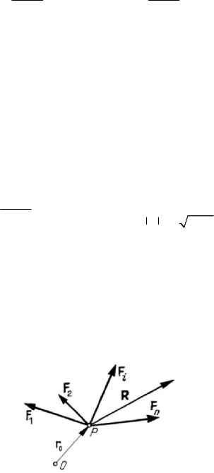
Figure 2.19. System of concentrated forces applied at the same point P .

Let

F be a discrete system of forces applied at a point

(

)

P r (concurrent forces)

(Fig.2.19); the equivalent fields are given by