Sundararaja D. The Discrete Fourier Transform. Theory, Algorithms and Applications

Подождите немного. Документ загружается.

324

Discrete Walsh-Hadamard Transform

Input

Vector

Formation

Stage 1

Output

Stage 2

Output

Stage 3

Output

x(0)

x(8)

*(1) [31

x(9) LU

x(2) m

ar(10)LU

x(3) [I

x(ll)[_0

x(4)

x(12)

x(5)

x(13)

x(6) fT|

x(14)LU

*(T)

x(15)liJ

E H

-2

-6

-8

-l

-2

-1

-4

-1

E i

3ll

(0)

9j X

nfe

(l)

{3)

Tl X

(4)

r9j

(5)

Til X

nft

(6)

U X„

(7)

FT] *nft(8)

LU *nh(9)

Fl X

(W)

^nh(H)

X„ft(12)

n7l

(13)

{U)

X„/>(15)

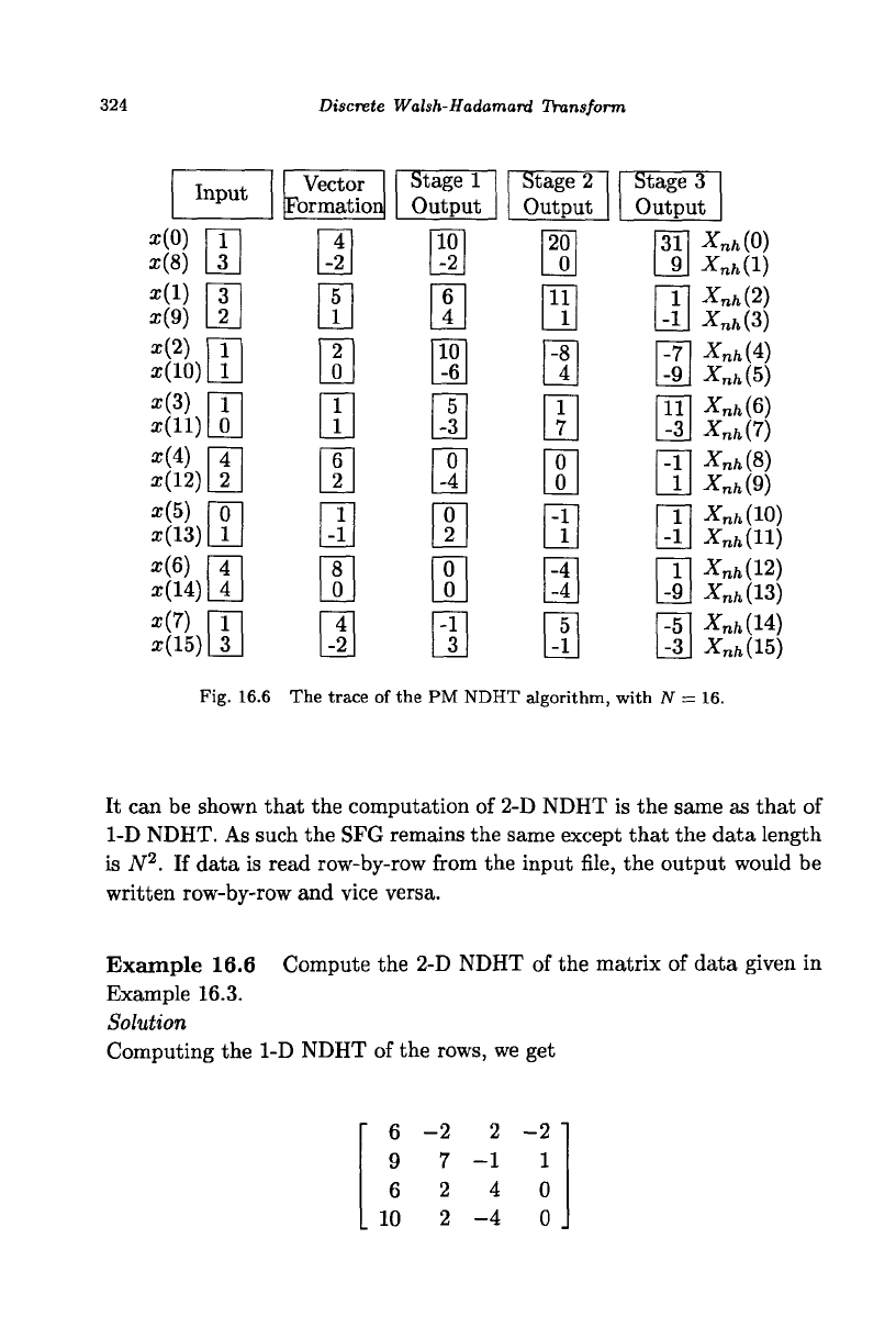
Fig. 16.6 The trace of the PM NDHT algorithm, with N = 16.

It can be shown that the computation of 2-D NDHT is the same as that of

1-D NDHT. As such the SFG remains the same except that the data length

is N

. If data is read row-by-row from the input file, the output would be

written row-by-row and vice versa.

Example 16.6 Compute the 2-D NDHT of the matrix of data given in

Example 16.3.

Solution

Computing the 1-D NDHT of the rows, we get

-2

-1

-4

-2

The Sequency Ordered Discrete Hadamard Transform 325

Computing

the 1-D

NDHT

of the

columns

of the

resulting matrix,

we get

fcl

->•

31 9

-7

-9

-1

-9

-5

-1

-3

-1

-3

The original image

can be

obtained

computing

the 1-D row

inverse

NDHTs of the transform matrix followed

by the 1-D

column inverse NDHTs

the

resulting matrix

and

vice versa.

16.3

The

Sequency Ordered Discrete Hadamard Transform

This transform generates

the

same sequency coefficients

that

of the

DWT,

but in

sequency-order ({0,1,1,2,2,3,3,4}

for N = 8). The

SDHT

data sequence {x(n),n

0,1,...,

—

1} is

defined

N-l

(k)

= £

x(n)(-l)^i=~

(fc)

0,1,...,

AT-1,

n=0

where

rii is the ith bit in the

binary representation

of n, the lsb is

indicated

the

subscript

0, and

(k)

= k

-i

9i {k)

= {k

-i + k

-2) mod 2

52(k)

= (&M-2 + k

s) mod 2

9M-I

(k) = (h +

)

mod 2

The matrix form

of the

defining equation, with

N = 8, is

written

(0)

{\)

{2)

(3)

(A)

(5)

(6)

(7)

1 1 1-1-1-1-1

1-1-1-1-1 1 1

1-1-1 1 1-1-1

1-1-1 1 1-1-1 1

1-1-1 1-1 1 1-1

1-1 1-1-1 1-1 1

1-1 1-1 1-1 1 -1

•

ar(0) "

x(l)

x{2)

x(3)

x(4)

x(5)

x(6)

*(7) .

326

Discrete Walsh-Hadamard Transform

"a 1

fe 0

CI 0

.. 00

& 1

•

"a 1

S. 0

^ 00

=s 1

•

(a)

(c)

• •

•

"e 1

5°

& -1

•

"s 1

C 0

.. 00

£ 1

•

"a 1 t»

!C 0

^ 00

fe 1

•

(b)

•

(d)

•

<•)

£ 0

& -1

(f)

1 M • • •

-1 L • . • . • . •.

(g) (h)

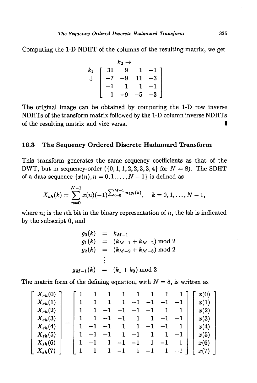
Fig. 16.7 The SDHT basis functions, with N = 8.

The SDHT basis waveforms,

(k,n)

= (-l)E";

"•»<(*), n,fc = 0,l,...,JV-l,

are shown in Fig. 16.7, with N — 8. It can be seen that the waveforms

are sequency ordered and are similar to the DFT basis waveforms. This

kernel can be obtained by rearranging the DWT kernel in gray-code order

(0,1,3,2,6,7,5,4, for

= 8). The inverse SDHT is given by

N_1

M-l

^ =

E *.ft(*)(-l)

-°

ni9i{k)

n =

0,1,...,

- 1

k=0

Example 16.7 Let x{n) =

{1,3,5,7}.

Compute the SDHT of x(n). Get

back x(n) by computing the inverse SDHT of the sequency coefficients.

The Sequency Ordered Discrete Hadamard Transform 327

Solution

(0)

(l)

(2)

(3)

The inverse SDHT is

x(0) = (16 + (-8) + (0) + (-4))/4 = 1

x(l) = (i6 + (-8)-(0)-(-4))/4 = 3

x{2) = (16 - (-8) - (0) + (-4))/4 = 5

*(3) = (l

-(-8) + (0)-(-4))/4 = 7 I

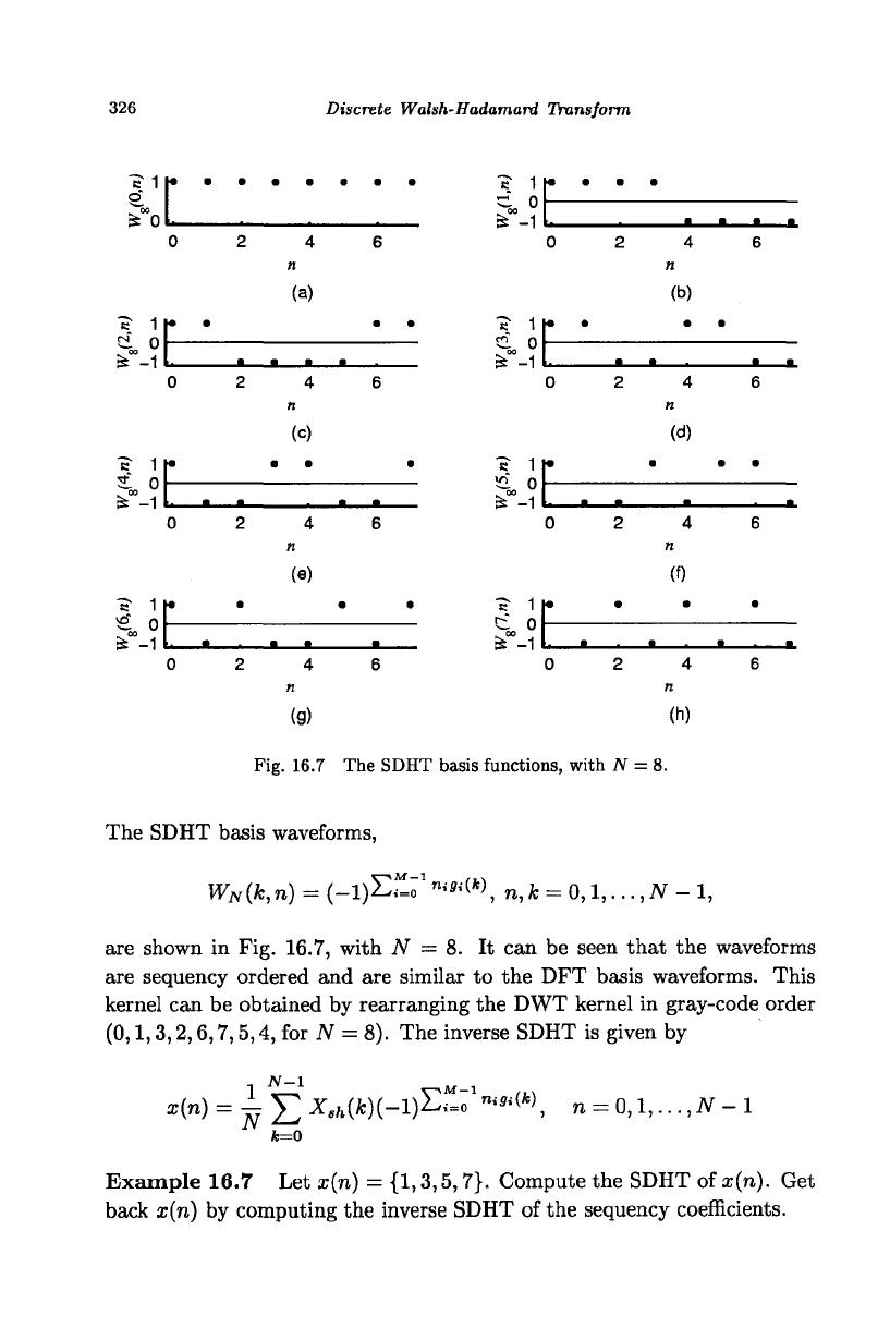
The PM SDHT algorithm

This algorithm is similar to the PM NDHT algorithm with the following

differences: (i) the input vectors are formed with a different pair of elements

and they are placed in the bit-reversed order and (ii) the output at the lower

node of a butterfly is stored in a different order. The input vectors a(n)

are defined as

a(n) = {a

(n),ai(n)} = {x{2n) + x{2n + l),x(2n) - x(2n + 1)},

n = 0,l,...,y-l

The output vectors A(k) are defined as

A(k) = {A

(k), A^k)} = {X

(2k),X

(2k + 1)}, fc =

0,1,...,

y - 1

The equations characterizing the PM SDHT butterfly are given as

r+1)

(/i)

= a£\h)+a£\l)

\h)

(/»)-4

r+1

\l) = a[

\h)-a[

\l)

af?

\l) = o[

(/i)+a[

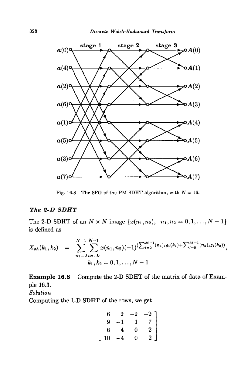
The SFG of the PM SDHT algorithm, with N = 16, is shown in Fig. 16.8.

= 1 + 3 + 5 + 7 = 16

= 1+3-5-7=-8

1-3-5+7=0

1-3+5-7=-4

328

Discrete Walsh-Hadamard Transform

o(0)

o(4)

o(2)

«(6)

o(l)

o(5)

o(3)

o(7)

stage 1 stage 2 stage 3

A(0)

A(l)

A(2)

A(3)

•A(4)

A(5)

A(6)

^(7)

Fig. 16.8 The SFG of the PM SDHT algorithm, with N = 16.

The 2-D SDHT

The 2-D SDHT of an JV x JV image {x(ni,n

), ni,n

0,1,...,

N - 1}

is defined as

*.*(*!,to) = £ E x(n

)(-l)

(

S";

("0^(fc

)+E"o

^)'^^»,

ni=0n2=0

fcl,fc

=0,l,...,JV-l

Example 16.8 Compute the 2-D SDHT of the matrix of data of Exam-

ple 16.3.

Solution

Computing the 1-D SDHT of the rows, we get

6 2-2-2

9-117

6 4 0 2

10-4 0 2

Summary

329

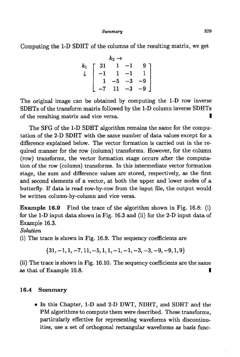
Computing the 1-D SDHT of the columns of the resulting matrix, we get

-»•

31 1-1 9 "

-1 1-1 1

1 -5 -3 -9

-7 11 -3 -9 .

The original image can be obtained by computing the 1-D row inverse

SDHTs of the transform matrix followed by the 1-D column inverse SDHTs

of the resulting matrix and vice versa. I

The SFG of the 1-D SDHT algorithm remains the same for the compu-

tation of the 2-D SDHT with the same number of data values except for a

difference explained below. The vector formation is carried out in the re-

quired manner for the row (column) transforms. However, for the column

(row) transforms, the vector formation stage occurs after the computa-

tion of the row (column) transforms. In this intermediate vector formation

stage, the sum and difference values are stored, respectively, as the first

and second elements of a vector, at both the upper and lower nodes of a

butterfly. If data is read row-by-row from the input file, the output would

be written column-by-column and vice versa.

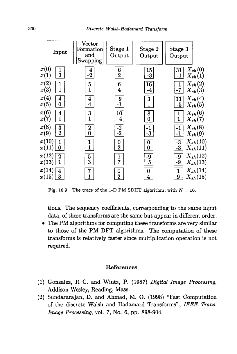
Example 16.9 Find the trace of the algorithm shown in Fig. 16.8: (i)

for the 1-D input data shown in Fig. 16.3 and (ii) for the 2-D input data of

Example 16.3.

Solution

(i) The trace is shown in Fig. 16.9. The sequency coefficients are

{31, -1,1, -7,11, -5,1,1, -1, -1,

-3, -3, -9, -9,1,9}

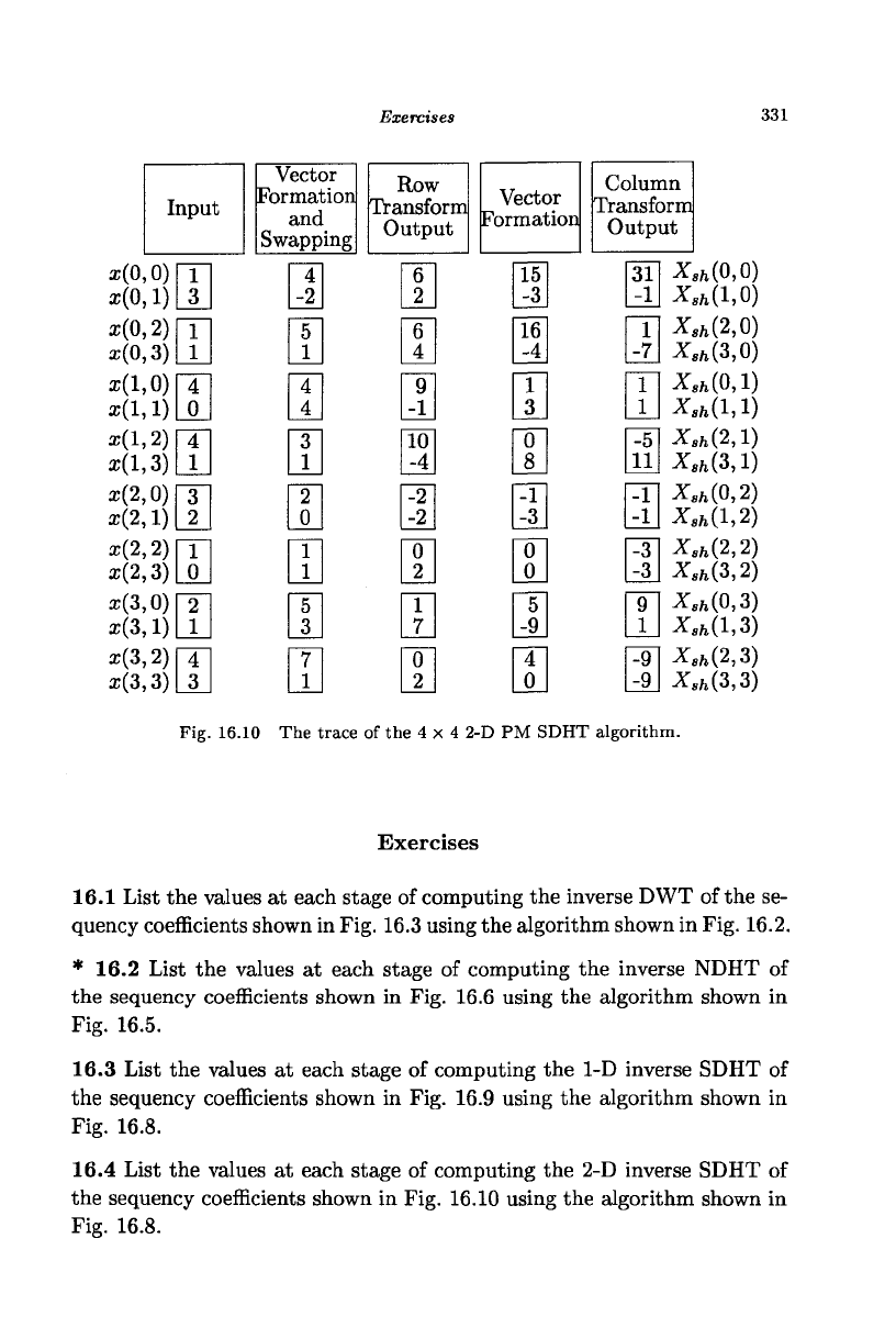
(ii) The trace is shown in Fig. 16.10. The sequency coefficients are the same

as that of Example 16.8. I

16.4 Summary

• In this Chapter, 1-D and 2-D DWT, NDHT, and SDHT and the

PM algorithms to compute them were described. These transforms,

particularly effective for representing waveforms with discontinu-

ities,

use a set of orthogonal rectangular waveforms as basis func-

330

Discrete Walsh-Hadamard Transform

Input

Vector

Formation

and

Swapping

Stage 1

Output

Stage 2

Output

Stage 3

Output

x{0

x(l

x(2

x (3

x (4

x(5

x(6

x(7

x(8

x(9

z(10)

z(ll)

*(12)

z(13)

a;(14)

x(15)

_3_

-1

-4

-2

-1

-3

a a

-9

3T1

(0)

Gn x

(i)

(2)

(3)

mn x

(4)

Lil x

(5)

(6)

nn Jf.fc(8)

(10)

(U)

(12)

Jf.h(13)

(14)

(15)

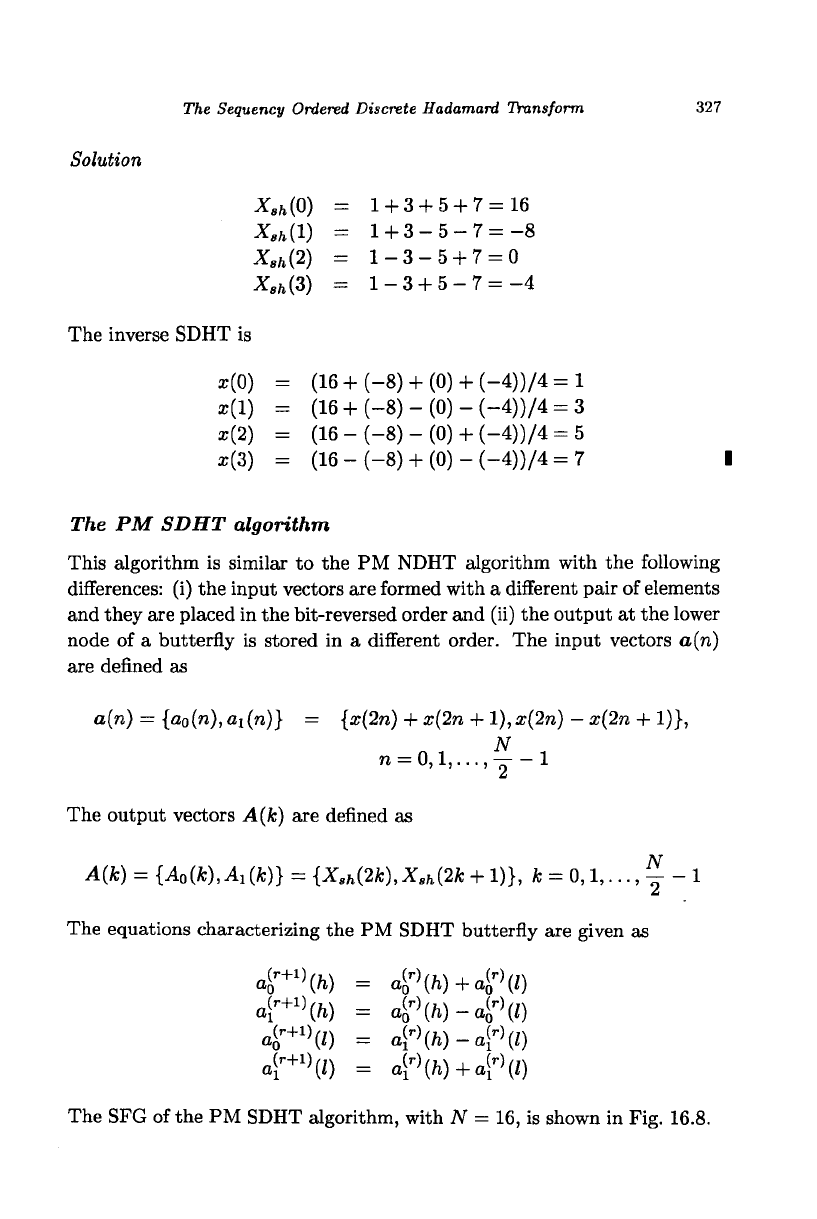
Fig. 16.9 The trace of the 1-D PM SDHT algorithm, with N = 16.

tions.

The sequency coefficients, corresponding to the same input

data, of these transforms are the same but appear in different order.

The PM algorithms for computing these transforms are very similar

to those of the PM DFT algorithms. The computation of these

transforms is relatively faster since multiplication operation is not

required.

References

(1) Gonzalez, R C. and Wintz, P. (1987) Digital Image Processing,

Addison Wesley, Reading, Mass.

(2) Sundararajan, D. and Ahmad, M. O. (1998) "Fast Computation

of the discrete Walsh and Hadamard Transforms", IEEE Trans.

Image Processing, vol. 7, No. 6, pp. 898-904.

Exercises

331

x(0, 0

X(0,

z(0,2

x(0,3

x(l,0

x(l,l

x(l,2

x(l,3

z(2,0

z(2,l

x(2,2;

a;(2,3

z(3,0

a;(3,1

z(3,2

z(3,3

Vector

Formation

and

Swapping

Row

Transform

Output

Vector

Formation

Column

Transform

Output

4 1

4 ]

-i

-4

-7

-4

-2

-1

-3

[-b\

-1

-9

-3

-9

fc(0,0

{\,Q

(Z,Q

{Q,\

(l,\

(2,l

h(3,1

s/l

(0,2

sft

(l,2

-X»fc(2,2

-^»fe(3,2

ft(0,3

^sfe(l,3

^«ft(2,3

^»/j(3,3

Fig. 16.10 The trace of the 4 x 4 2-D PM SDHT algorithm.

Exercises

16.1 List the values at each stage of computing the inverse DWT of the se-

quency coefficients shown in Fig. 16.3 using the algorithm shown in Fig. 16.2.

* 16.2 List the values at each stage of computing the inverse NDHT of

the sequency coefficients shown in Fig. 16.6 using the algorithm shown in

Fig. 16.5.

16.3 List the values at each stage of computing the 1-D inverse SDHT of

the sequency coefficients shown in Fig. 16.9 using the algorithm shown in

Fig. 16.8.

16.4 List the values at each stage of computing the 2-D inverse SDHT of

the sequency coefficients shown in Fig. 16.10 using the algorithm shown in

Fig. 16.8.

332 Discrete Walsh-Hadamard Transform

Programming Exercises

16.1 Write a program to implement the PM DWT algorithm.

16.2 Write a two stages at a time program to implement the PM DWT

algorithm.

16.3 Write a program to implement the PM NDHT algorithm.

16.4 Write a two stages at a time program to implement the PM NDHT

algorithm.

16.5 Write a program to implement the PM SDHT algorithm.

16.6 Write a two stages at a time program to implement the PM SDHT

algorithm.

16.7 Write a two stages at a time program to implement the 2-D PM SDHT

algorithm.

Appendix A

The Complex Numbers

The real number system can be represented by a number line. A real

number is the coordinate of a point on the line. Zero is the reference number

and the numbers to the right of zero are called positive numbers and those

to the left are called negative numbers. With this number system, we can

specify a movement along the line. Now, the question is how to specify a

movement along any direction, that is a movement in a plane. If we draw

another number line at right angles to our original number line, we can

specify any movement in the plane with the help of a pair of numbers, one

number taken from each line.

Using pairs of ordered numbers, taken from two perpendicular num-

ber lines, to represent points in a plane is the complex number system.

Although it is not really complex, unfortunately, it is called the complex

number system and a number is called complex number. Notwithstanding

the fact that each of the pair of numbers is just a real number, the first one

is called the real part and the second one is called the imaginary part of

the complex number. The plane formed by the two number lines is called

the complex plane. The first and the second number lines are called, re-

spectively, the real and imaginary axis of the complex plane. These names

are totally misleading and there is nothing complex or imaginary in repre-

senting a point in a plane with a pair of real numbers.

We stress this point so much because our principal object in Fourier

analysis, the sinusoid, is most efficiently represented by a point moving in

a plane. A pair of ordered real numbers is our standard denomination.

By using complex numbers, we manipulate sinusoids with manipulation of

numbers which is just little bit more involved than real numbers rather

333