Skiadas C.H., Skiadas C. Chaotic Modelling and Simulation. Analysis of Chaotic Models, Attractors and Forms

Подождите немного. Документ загружается.

34 Chaotic Modelling and Simulation

Probably the most well-known example of this type is the equation for the kinetic

energy of a mass. If f (v) represents the energy of the system, then a good approxi-

mation for small v (close to 0) would be:

f (v) = a

+ a

The two terms can be identiﬁed physically as the energy at rest

f (0) = a

and the kinetic energy

kin

= a

On the other hand, economic, social and biological phenomena do not have this

isotropic property. The same lack of symmetry holds for the time space, and the

relevant Taylor approximations tend to include a linear term as well. The constant

term in such a system can often be assumed to be zero.

Hence, a simple approx-

imation will involve linear and quadratic terms. This approximation gives rise to a

diﬀerential equation known as “The Logistic,” ﬁrst proposed by Verhulst (1845) to

model the population growth in France. Later on, Pearl and Reed (1920) applied this

model to express the population growth in the United States.

The logistic diﬀerential equation has the simple form

˙x = bx(1 − x) (2.9)

where x is the population at the present time, over the maximum level that the popu-

lation could reach in the future. In other words, x is the saturation level.

To see how equation (2.9) follows naturally from (2.6) through the process of a

Taylor series approximation, consider that x is restricted in the interval [0, 1]. We

can consider the value x =

where the population is at half its potential as the

centre, and assume that the system will exhibit symmetry around x =

. In that case,

the Taylor approximation to the second order would be:

f (x) = a

+ a

x −

− a



x − x



= a + bx(1 − x)

Here a is the rate of growth of the population when the population is at x = 0 or

x = 1, so we can reasonably assume that a = 0. The other parameter, b, is related to

the growth rate at x =

. We are thus led to equation (2.9).

Equation (2.9) is a separable diﬀerential equation, and so can be easily solved

explicitly, by rewriting it as

x(1 − x)

dx = bdt

For instance in birth processes or innovation diﬀusion cases.

Models and Modelling 35

The solution then would satisfy:

−ln(1 − x) + ln(x) = bt + C

This last equation can be rewritten in the ﬁnal form:

x(t) =

1 + x



− 1



(2.10)

The graph of (2.10) exhibits a very characteristic smooth sigmoid form (Fig-

ure 2.1).

−6 −4 −2 0 2 4 6

x((t)) ==

1 ++ x

((e

−− 1))

FIGURE 2.1: The solution to the logistic equation

A diﬀerence equation whose form closely parallels that of equation 2.9, but whose

behaviour is a lot more interesting, also goes under the name “logistic”:

t+1

= bx

(

1 − x

)

(2.11)

The behaviour of the solutions to (2.11) depends on the value of the parameter b.

When b < 3, they follow a discrete sigmoid form. However, when b > 3 chaotic

oscillations appear. The oscillations become progressively more chaotic as b ap-

proaches 4. The behaviour of the solutions of the discrete logistic will be explored

further in Chapter 3.

The correct diﬀerence equation analogue to (2.11), using the approximation of the

ﬁrst derivative by a ﬁnite diﬀerence as in (2.2), is:

t+1

= x

+ bx

(1 − x

)

Various second, third and higher order forms of diﬀerential and diﬀerence equa-

tions models can be constructed with similar methods as above. These equations

may in some cases exhibit chaotic behaviour. These models will be examined more

closely in subsequent chapters.

36 Chaotic Modelling and Simulation

2.3.2 Empirical model formulation

In many cases in Physics, Biology, Economics, Marketing, Forecasting, etc, the

construction of an appropriate general model follows by the empirical investigation

of realistic situations. For instance, when the growth rate ˙x is assumed to be propor-

tional to the magnitude x of the system, then we end up with the exponential model

discussed on page 31. Another example is based on the relative growth rate

˙x

ln x = (ln x)

′

= ˙y

where y, the relative magnitude of the system, is deﬁned as

y =

= ln x

and can be approximated by

y ≈

∆x

That is, the relative magnitude y is a measure of all the relative changes of the system

from its original formation until its current status.

In this case, the standard measure of growth is the relative magnitude of the sys-

tem, which is assumed as the metric scale of the system. This assumption leads to

a convenient model construction especially when systems measured in completely

diﬀerent scales are to be compared. Examples of using the relative magnitude of

the system as the standard measure are the Gompertz, Gaussian and Gamma models,

whose descriptions follow.

2.3.2.1 The Gomp ertz model

The simplest assumption about the relative growth rate is that it is constant. This

leads us to the exponential growth model

˙x

= b discussed already. However, as it is

reasonable to expect that a system has limits to its growth, it would be more realistic

to assume a declining relative growth rate. Assuming that this decline is proportional

to the relative growth y of the system, we are led to a simple diﬀerential equation in

˙y = −by (2.12)

(ln x)

′

= −b ln x (2.13)

which can ﬁnally be rewritten as:

˙x = −bx ln x (2.14)

This model was ﬁrst proposed in Gompertz (1825). Direct integration gives as

solution the Gompertz function:

x = e

ln(x

−bt

Models and Modelling 37

Using the Taylor approximation methods of section 2.3.1, we can examine the

Gompertz system near x = 1: The logarithm ln(x) can be approximated by:

ln(x) ≈ x − 1

Using this approximation in (2.14) would result exactly in the logistic model. So for

x near 1, the Gompertz model can be approximated by the logistic model.

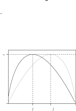
Another interesting variant occurs if we replace x by 1 − x in the Gompertz diﬀer-

ential equation, resulting in:

˙x = −b(1 − x) ln(1 − x)

This model arises by considering the relative decay of the system, instead of the

relative growth. This model has skewness opposite to that of the Gompertz model,

as now the maximum growth rate is achieved when

x = 1 −

instead of when x =

. A comparison of the two models is given in Figure 2.2.

Both models are referred to in the literature as “the Gompertz model,” with diﬀerent

disciplines preferring one model over the other. The second variant is favoured in

the actuarial sciences, as it is more intimately related to mortality.

1 e 1 −− 1 e

⋅⋅

FIGURE 2.2: The two Gompertz models

2.3.2.2 The Gaussian and Gamma models

The well familiar Gaussian and Gamma distributions arise naturally from the

relative-growth-rate setting, after some rather reasonable assumptions. For instance,

if may assume that the relative growth rate is a linear function of time, which leads

38 Chaotic Modelling and Simulation

us to the following equation:

˙y = (ln x)

′

= a − bt (2.15)

where b > 0.

The solution to (2.15) is a Gaussian function, namely:

x = ce

−

(t−µ)

2σ

where µ =

, σ

= b, and the integration constant c is determined by normaliza-

tion.

If, on the other hand, one assumes a slightly diﬀerent decreasing pattern for the

relative growth rate:

˙y = (ln x)

′

= a(ln t)

′

− λ

then the solution is related to the Gamma function:

x = c(λt)

−λt

2.3.3 The calculus of variations approach

Calculus of variations is concerned with optimising a functional:

I =

L( ˙x, x, t) dt (2.16)

where the functional L, called the Lagrangian, summarises the dynamics of the sys-

tem in question, in terms of ˙x, x and t. The ﬁrst step in the modelling process in this

case is the construction of an appropriate Lagrangian function. The solution to the

optimisation problem is then given by the Euler-Lagrange equation:

∂L

∂ ˙x

−

∂L

∂x

= 0 (2.17)

As a speciﬁc example, suppose the Lagrangian consists of two basic components:

L( ˙x, x, t) = G( ˙x) + V(x)

where G( ˙x) expresses the forces of growth, and V(x) expresses the limits of the

system. Then the Euler-Lagrange equation becomes:

∂G( ˙x)

∂ ˙x

−

∂V(x)

∂x

= 0 (2.18)

The form of the functions G( ˙x) and V(x) is not always known. However, as the

integral (2.16) involves a summation of the inﬁnitesimal parts of a path, it is in many

cases valid to approximate the functions G( ˙x) and V(x) using Taylor series, especially

when the growth system is continuous and smooth.

Models and Modelling 39

Note further an interesting property of equation (2.18): The ﬁrst order term of

a Taylor series expansion of G( ˙x) does not contribute to the equation. Hence, the

simplest expression for G ( ˙x) is ˙x

, and this is suﬃcient in many systems. This as-

sumption leads to a Lagrangian of the form

L =

˙x

+ V(x)

Equation (2.17) yields, in this case, the following diﬀerential equation of growth:

¨x =

∂V

∂x

(2.19)

The simplest interesting expression for V is V(x) =

. Equation (2.19) then

takes a very familiar form:

¨x = bx

When b > 0, this model expresses a growth process, while when b < 0, it expresses

an oscillating process.

If we consider the Lagrangian as a function of the relative growth rate of a system,

y = ln x, then the exact same analysis will yield the equation:

¨y =

∂V

∂y

Assuming V is constant, V(y) = c, we are led to the exponential model:

¨y = 0 ⇒ ˙y = b ⇒ (ln x)

′

= b ⇒ ˙x = bx

As we’ve seen before, when b < 0 this equation expresses a decay process.

2.3.4 The probabilistic-stochastic approach

A lot of models have their roots in probabilistic-stochastic considerations, which

give rise to certain partial diﬀerential equations. These are usually diﬀusion equa-

tions. The simple diﬀusion equation (D is the diﬀusion coeﬃcient)

∂u

∂t

= D

∂

∂x

and the Fokker-Planck equation

∂u

∂t

= −

∂(au)

∂x

+ D

∂

∂x

are the basis for many models.

A reaction-diﬀusion equation has the general form

∂u

∂t

= f (u) + D∇

40 Chaotic Modelling and Simulation

where, as usual, the Laplacian ∇

is given by:

∇

≡

∂

∂x

∂

∂y

∂

∂z

A classical model of this type is the so-called FitzHugh-Nagumo model (FitzHugh,

1961, 1969; Nagumo et al., 1962). The one-variable form of this model is given by

˙u = u(1 − u

) + K + D∇

where K is a parameter.

Simulation of models of this type gives rise to important chaotic cases of pattern

formation. These models explain the development of chaotic waves in ﬂuids and

chemical kinetics.

2.3.5 Delay growth functions

Delay growth models assume that the rate of growth, ˙x =

, is a function not only

of (x, t), but also of some earlier time (t −T ), where T is the delay. The general form

for a continuous ﬁrst-order delay growth model is:

˙x = f



x, (t − T ), t



A very simple delay growth model is the following multiplicative process:

˙x = bx

t−T

g(x

) (2.20)

Equation (2.20) is not easy to handle. However, an approximation of the delay

term is possible if we retain the ﬁrst two terms of a Taylor series expansion at t:

t−T

≈ x

− T ˙x (2.21)

Substituting (2.21) in (2.20) and rearranging terms, we obtain the system:

˙x =

bxg(x)

1 + bT g(x)

Depending on the the function g(x), many diﬀerent models arise. If, for instance,

g is set to be the decreasing function g(x) = 1 − x, then we obtain the GRM1 model

proposed in Skiadas (1985) to express an innovation diﬀusion process:

˙x =

bx(1 − x )

σ + (1 − σ)x

(2.22)

where σ = 1 + bT . When no delay is present, σ = 1 and (2.22) reduces to the logistic

diﬀerential equation (2.9).

The discrete alternatives of delay growth models, expressed by diﬀerence equa-

tions, give chaotic solutions for certain parameter values. These are examined in

some detail in Chapter 4.

Models and Modelling 41

2.4 Chaotic Analysis and Simulation

In the past decades, extensive studies in various ﬁelds led to the creation of a

new ﬁeld of analysis, called “Chaotic Analysis.” The innovation of this new ﬁeld

lies in its multidisciplinary approach to the problems studied, and its use of vari-

ous methods and tools not applied before. Most notable among these is the use of

computers for the related analysis and simulation, that has become an integral part

of Chaotic Analysis. Determining the number of equilibrium islands and their loca-

tions inside a chaotic sea is done ﬁrst by using chaotic simulations, and only later

by exact calculations, when possible. If we exclude computers and simulations from

chaotic analysis, an essential part of the chaotic phenomena, “the essence of chaos”

according to Lorenz (Lorenz, 1993), will be lost.

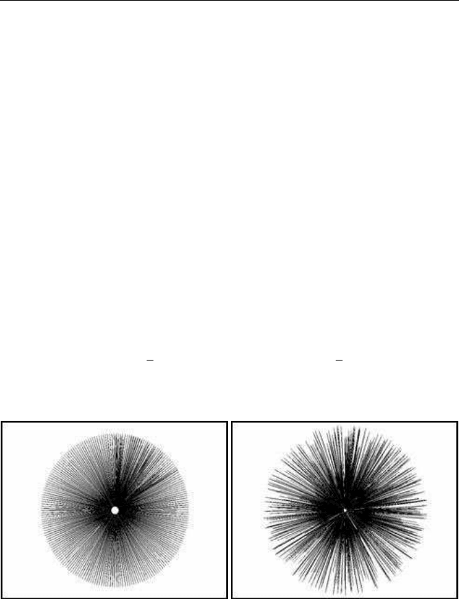
As an example of the advantages of simulation, consider the following formation

of two variants of a two-dimensional sea urchin, by using the logistic diﬀerence

equation and a simple rotation scheme. The equations used are:

t+1

= b f

(1 − f

)

= (1 − f

) cos(θ

)

= (1 − f

) sin(θ

)

(2.23)

The rotation angle θ

changes by h = 0.01 in each time step, and the chaotic para-

meter b is set to b = 1 +

√

8 in Figure 2.3(a) and b = 1.1 +

√

8 in Figure 2.3(b).

(a) (b)

FIGURE 2.3: Chaotic forms

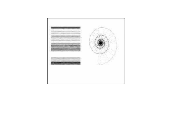
The shape of a snail is formed from the same logistic diﬀerence equation as above,

but now the chaotic band (t, f ), which appears on the left side of Figure 2.4, rotates

42 Chaotic Modelling and Simulation

and simultaneously sinks, due to the addition of an exponential decay factor, in order

to form the two-dimensional shape of a snail (right). The system of equations used

is:

t+1

= b f

(1 − f

)

= (1 − f

) cos(θ

−at

= (1 − f

) sin(θ

−at

(2.24)

The chaotic parameter used here is 1.03 +

√

8, and the time step is h = 0.005.

FIGURE 2.4: A snail’s pattern

2.5 Deterministic, Stochastic and Chaotic Models

Deterministic models are expressed by speciﬁc, deterministic equations, which

give the same results for the same initial conditions. Stochastic models on the other

hand are given by stochastic equations, which may give diﬀerent paths, and dif-

ferent ﬁnal results, for the same initial conditions. The chaotic models can act as

deterministic models for some parameter values, but for some other values of the

chaotic parameters they will give radically diﬀerent ﬁnal values for inﬁnitesimally

small changes in the initial values. Chaotic models are in a sense deterministic, in

that the ﬁnal values are determined completely from the precise initial values. From

a practical point of view however, given the sensitivity of chaotic models to the ini-

tial conditions, the unpredictability of the ﬁnal results and the non-uniqueness of the

paths followed by the system in chaotic systems are in some ways similar to the

unpredictability and non-uniqueness present in stochastic models.

As an illustration of this idea, one could attempt to use the logistic model as a

random number generator. To achieve that, consider the one-dimensional stochastic

Models and Modelling 43

process generated by the following set of diﬀerence equations:

t+1

= 1 −2x

t+1

= y

+ ex

(2.25)

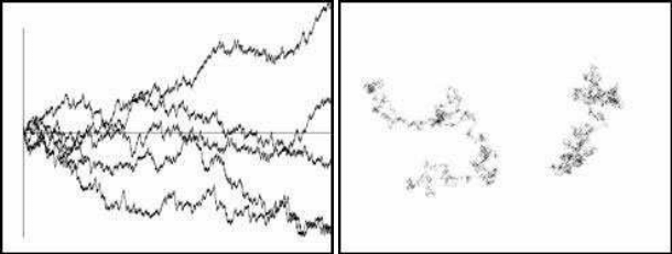
Here, e is a small parameter (e = 0.17). Several paths of this process are illustrated in

Figure 2.5(a). The resemblance of these paths to those of a Wiener process is strik-

ing. Another example, reminiscent of Brownian motion, appears in Figure 2.5(b).

This ﬁgure shows a two-dimensional stochastic process based on a four-dimensional

mapping.

(a) One-dimensional diﬀusion (b) Two-dimensional diﬀusion

FIGURE 2.5: Chaos as randomness