Skiadas C.H., Skiadas C. Chaotic Modelling and Simulation. Analysis of Chaotic Models, Attractors and Forms

Подождите немного. Документ загружается.

4 Chaotic Modelling and Simulation

(a) The continuous case (x, y) (b) A discrete analogue

FIGURE 1.2: Continuous and discrete R

ossler systems

1.2 Chaos in Diﬀerence Equation Systems

Radical changes in the behaviour appear when a system of diﬀerential equations is

replaced by a similar system of diﬀerence equations, or by a single diﬀerence equa-

tion with non-linear terms. For example, suppose we replace the R

ossler system (1.4)

by a corresponding system of diﬀerence equations:

t+1

= x

−

+ z

)

t+1

= y

t+1

+ ey

)

t+1

= z

+ 0.1 + ex

t+1

(1.5)

Then, for parameter value e = 0.2, and iterating under the condition x

t+1

= x

− 0.4,

an interesting chaotic form like a sea-shell results (Figure 1.2(b)).

For centuries the mathematical development of methods and tools of analysis con-

centrated mainly on diﬀerential equations, and not on diﬀerence equations. It is

therefore not surprising that the logistic model, the most popular chaotic diﬀerence

equation model today, was “invented” only in the last three decades. The logistic

model is described by a very simple equation:

t+1

= bx

(1 − x

) (1.6)

This very simple model already exhibits the key elements of chaotic behaviour. As

the parameter b increases, period doubling bifurcations occur, giving rise to stable

orbits of ever increasing size, culminating in completely chaotic behaviour. On the

other hand, the diﬀerential equation analogue of this model was very popular:

˙x = bx(1 − x) (1.7)

Introduction 5

Equation (1.7), as expected, gives simple ﬁnite solutions without complications

and chaotic behaviour. This continuous model, called the logistic model, was applied

in demography by Verhulst already in 1838.

Chapter 2, further discusses models and the modelling process in general. Deter-

ministic, stochastic and chaotic models are introduced, along with chaotic analysis

and simulation techniques. The subsequent chapters deal with particular classes of

models, and their interesting behaviour.

1.2.1 The logistic map

Chapter 3 is devoted to a detailed analysis and simulation of the chaotic behaviour

of non-linear diﬀerence equations, starting with the logistic model. The logistic map

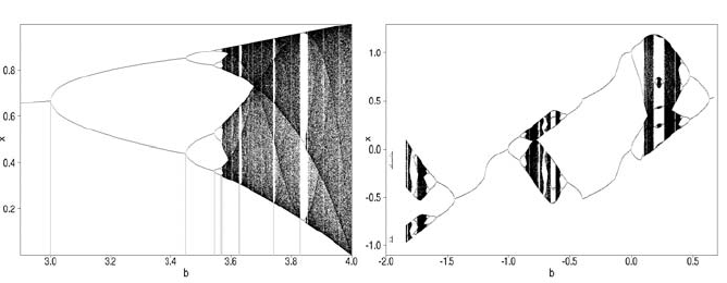
and its bifurcation diagram are presented. The bifurcation diagram exhibits the stable

orbit of the x values for each value of the chaotic parameter b. In the case of the

logistic model, the stable orbits become more and more complex as b increases,

culminating in the complete chaos observed for b close to 4.

Other models that are examined, and exhibit similar behaviour, are: the sinusoidal

model, the Gompertz model and a model proposed by May. Also, a class of models

with behaviour diﬀerent than that of the quadratic maps are studied, the Gaussian-

type models. As can be seen clearly from the bifurcation diagrams of the logistic

(Figure 1.3(a)) and the Gaussian model (Figure 1.3(b)), there are clear diﬀerences

between the two classes of models, as well as some similarities in the chaotic win-

dows.

(a) Logistic (b) Gaussian

FIGURE 1.3: Bifurcations of the logistic and the Gaussian

6 Chaotic Modelling and Simulation

1.2.2 Delay models

Delay models are models where future values depend on values far in the past. For

instance, a simple delay equation is the delay logistic:

t+1

= bx

(1 − x

t−m

)

which is analysed further in Chapter 4, along with some variations and more com-

plicated models.

Delay models can be found in several real life cases when the future development

of a phenomenon is inﬂuenced from the past. The complexity of the delay system

is higher when the delay is large and the equations used are highly non-linear. Such

chaotic behaviour is expressed by a model proposed by Glass

t+1

= cx

+ a

t−m

1 + x

t−m

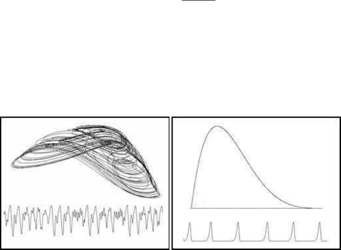
When the parameters are a = 0.2, c = 0.9 and the delay m = 30, the Glass model

gives a very complicated graph in the phase space and chaotic time oscillations of a

very complex character (Figure 1.4(a)). Figure 1.4(b) presents the map of the delay

logistic, as well as the related oscillations, when the delay is m = 10. The chaotic

parameter is b = 1.2865.

(a) The Glass model (b) The delay logistic

FIGURE 1.4: Delay models

1.2.3 The H´enon model

In some cases a system of two diﬀerence equations is replaced by a single dif-

ference delay equation with the same properties. This is the case of the H

enon

Introduction 7

model (H

enon, 1976), which can be thought of either as a system of two diﬀerence

equations, or as a single delay equation. The model proposed by H

enon, which is

now considered one of the standard models in the chaos literature, has the form:

t+1

= 1 −ax

+ y

t+1

= bx

(1.8)

The equivalent delay diﬀerence equation of the H

enon system is:

t+1

= bx

t−1

+ 1 − ax

(1.9)

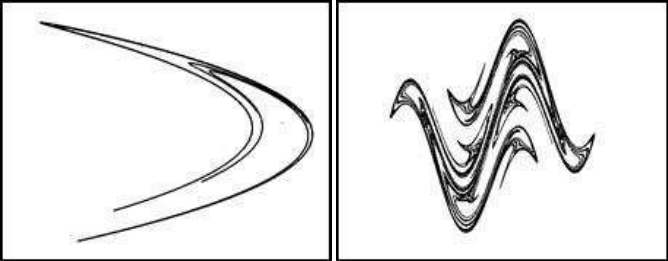
For parameter values a = 1.4 and b = 0.3 the famous H

enon attractor is formed

(Figure 1.5(a)).

(a) The H

enon attractor (b) The Holmes attractor

FIGURE 1.5: The H

enon and Holmes attractors

Another model, with very interesting properties, was proposed by Holmes (Holmes,

1979a):

t+1

= bx

t−1

+ ax

− x

(1.10)

Fig 1.5(b) presents the Holmes model when the parameters take the values a = 3, b =

0.8.

The H

enon model, along with other related models, extensions and variations,

such as the Holmes model, are presented in Chapter 5.

8 Chaotic Modelling and Simulation

1.3 More Complex Structures

1.3.1 Three-dimensional and higher-dimensional models

A number of interesting three-dimensional models are studied in Chapter 6. These

include the Lorenz (Lorenz, 1963) and R

ossler models, the autocatalytic and Ar-

neodo (Arneodo et al., 1980, 1981b) models, and their extensions and variations.

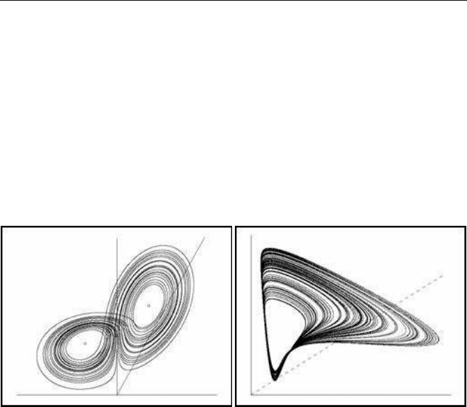
3-dimensional views of the Lorenz and autocatalytic attractors are illustrated in Fig-

ures 1.6(a) and 1.6(b) respectively.

(a) The Lorenz attractor (3-d) (b) The autocatalytic attractor

FIGURE 1.6: The Lorenz and autocatalytic attractors

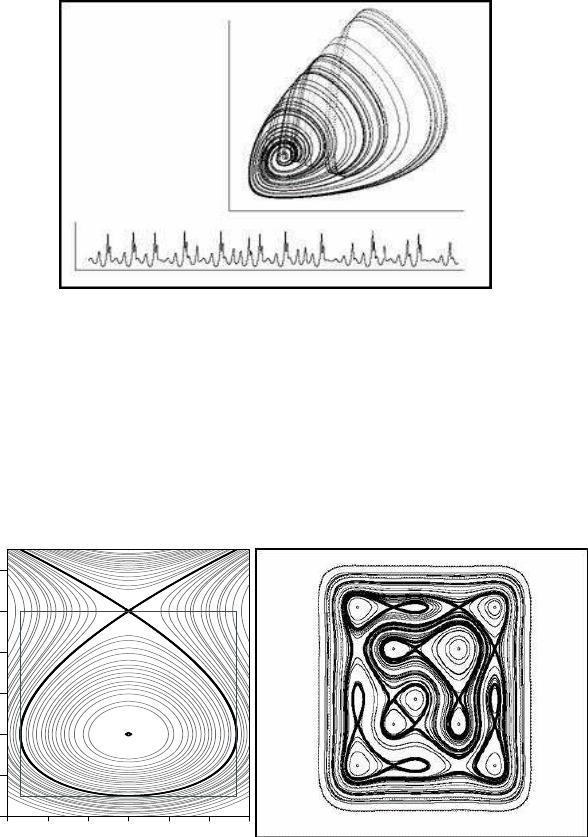
We also examine a four-parameter model of chemical reactions, which gives rise

to a rich variety of chaotic patterns. A two-dimensional view of this chaotic at-

tractor, along with the time development of one-dimensional oscillations, appears in

Figure 1.7.

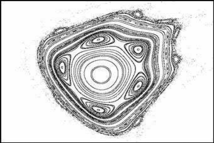
1.3.2 Conservative systems

In Chapter 7, we consider conservative systems, that is, systems that have a non-

trivial ﬁrst integral of motion, and in particular Hamiltonian systems. The existence

of a ﬁrst integral of motion provides enough information to draw the phase portrait of

the system in cartesian coordinates. The resulting patterns exhibit a varying degree of

symmetry, depending on the equations of the system. Figure 1.8 shows an example

of two of the forms analysed in this chapter.

Introduction 9

FIGURE 1.7: A chemical reaction attractor

−0.3 −0.2 −0.1 0.0 0.1 0.2 0.3

−0.4

−0.2

0.0

0.2

0.4

0.6

0.8

FIGURE 1.8: Non-chaotic portraits

10 Chaotic Modelling and Simulation

1.3.3 Rotations

Chapter 8 is devoted to rotations, reﬂections and translations, and the chaotic

forms and attractors that these give rise to. The models in this category are char-

acterized by the presence of rotations and translations, as well as non-linear terms,

in the system equations. For appropriate values of the parameters, these models give

rise to chaotic patterns and attractors. The most popular of these is probably the

Ikeda model (Ikeda, 1979) (equations (1.14) and (1.13)).

Rotation models express a large variety of systems in various disciplines. A simple

rotation in the plane, followed by a translation, does not in itself lead to chaotic

forms. The rotation equation, in its usual form, is based on linear functions such

as (1.11):

t+1

= x

cos(θ

) − y

sin(θ

)

t+1

= x

sin(θ

) + y

cos(θ

)

(1.11)

However, the introduction of non-linear terms in system (1.11) gives chaotic so-

lutions. First of all, let us consider the eﬀect of adding a quadratic term in both

equations. The system then becomes non-linear:

t+1

= x

cos(θ) − y

sin(θ) + x

sin(θ)

t+1

= x

sin(θ) + y

cos(θ) − x

cos(θ)

(1.12)

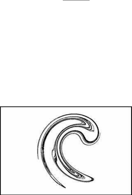
When the rotation angle is stable, θ = 1.3, the system gives an interesting two-

dimensional map with chaotic regions and islands of stability inside these regions

(Figure 1.9).

FIGURE 1.9: A rotation chaotic map

Another way to add non-linearity is to assume that the rotation angle θ is a non-

linear function, as is the case of the famous Ikeda attractor. The model is based on

a system of two rotation equations with a translation parameter a added to the ﬁrst

Introduction 11

equation, a space parameter b, and a non-linear rotation angle of the form:

= c −

1 + x

+ y

(1.13)

The rotation-translation system in this case takes the following form:

t+1

= a + b



cos(θ

) − y

sin(θ

)



t+1

= b



sin(θ

) + y

cos(θ

)



(1.14)

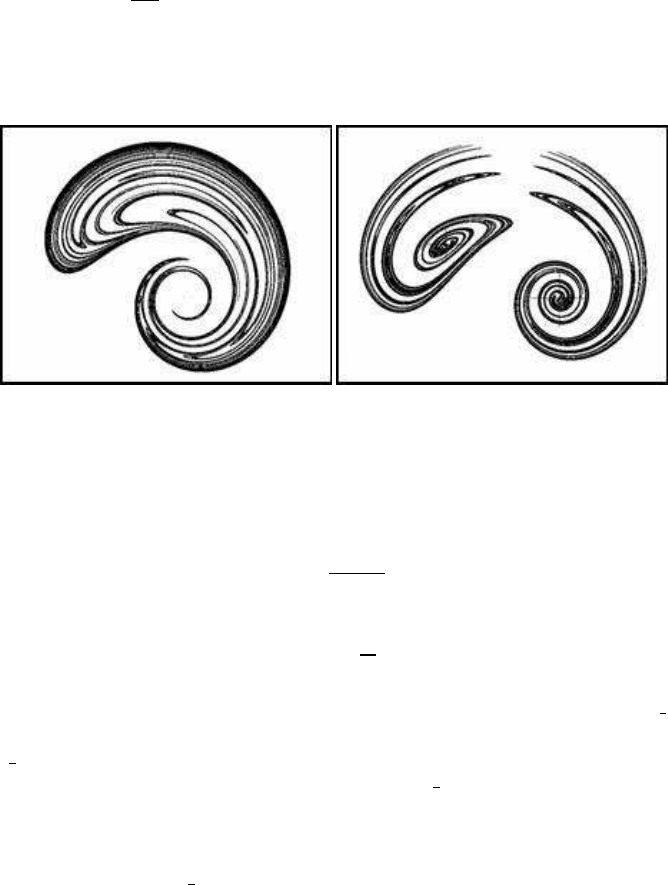
This system was ﬁrst proposed by Ikeda (1979) to explain the propagation of light

into a ring cavity. The parameter values in that case where a = 1, b = 0.83, c = 0.4

and d = 6, and they give rise to a very interesting attractor illustrated in Figure 1.10.

FIGURE 1.10: The Ikeda attractor

This map has Jacobian J = b

. When b < 1 several chaotic and non-chaotic

patterns can be seen in the various simulations, some of which are illustrated in

Chapter 8.

The properties of the chaotic maps in this category are so rich and often unex-

pected. The shape of the Ikeda attractor in the previous standard form depends on

the selection of the values of the parameters. By varying these parameters, very inter-

esting new forms appear. A wide variety of these forms are presented and analysed

in Chapter 8. Two of these attractors are illustrated in Figures 1.11(a) and 1.11(b). In

Figure 1.11(a) an attractor pair appears. The parameters are a = 6, b = 0.9, c = 3.1

and d = 6. In Figure 1.11(b), only the parameter c is changed (c = 2.22). Now three

images of the attractors are present.

12 Chaotic Modelling and Simulation

(a) A double Ikeda attractor (b) A triple Ikeda attractor

FIGURE 1.11: Ikeda attractors

1.3.4 Shape and form

In Chapter 9 we study how chaotic analysis can be used as a tool to design forms

that appear in physical systems. Such an analysis is useful in the scientiﬁc ﬁeld re-

lated to shape and form. Even the most strange chaotic attractors and forms can have

real signiﬁcance, especially in biological systems but also in ﬂuid ﬂow or in crys-

tal formation. The analysis of these systems has moved from the classical analysis

concerning simple and regular forms to chaotic analysis. The aim here is to go be-

yond the classical stability analysis. We try to ﬁnd mechanisms to design simple or

complicated and chaotic forms, and to pass from a qualitative to a quantitative point

of view. The sea-shell formation illustrated earlier in this chapter is one case of an

attractor with a special shape. The equations used are 3-dimensional and the original

inspiration comes from the R

ossler model.

The main tools for shape formation are rotation and translation, as in the Ikeda

case above, but also reﬂection with translation, based on the following set of equa-

tions:

t+1

= a + b



cos(2θ

) + y

sin(2θ

)



t+1

= b



sin(2θ

) − y

cos(2θ

)



(1.15)

If the same function as in the Ikeda case is used for the angle θ

= c −

1 + x

+ y

then we obtain an attractor (Figure 1.12(a)) which is divided in two new separate

forms (Figure 1.12(b)). The parameters in the ﬁrst case are a = 2.5, b = 0.9, c = 1.6

and d = 9. In the second case, a = 6 and the other parameters remain unchanged.

Introduction 13

The centres of the two attractors are located at:

(x, y) = (a, 0) and

(x, y) =



a + ab cos(θ), ab sin(θ)



where θ = c −

1+a

. The reﬂection attractor is on the left side of Figure 1.12(b).

These cases simulate the split of a vortex in two separated forms. The parameter a is

quite higher than in the previous case.

(a) Reﬂection with 1 image (b) Reﬂection with 2 images

FIGURE 1.12: Translation-reﬂection attractors

The rotation equation (1.14), applied to the Ikeda case, but now with b = 1, is a

space-preserving transformation. Interesting forms arise assuming that the rotation

angle is a function of the distance r

+ y

. For instance, when

= c +

we obtain the form illustrated in Figure 1.13(a). There is a symmetry axis at x =

and one equilibrium point in the central part of the ﬁgure, located at

(

x, y

t+1

)



, y



. The ﬁve equilibrium points in the periphery are of the ﬁfth order:

(

t+5

, y

t+5

)

(

, y

)

. One of these points is also located on the x =

axis, whereas the other four

are located in symmetric places about this axis. The parameters are a = 3, c = 1 and

d = 4.

Furthermore, the Ikeda model with b = 1 provides interesting forms with the same

axis of symmetry, x =

. Figure 1.13(b) illustrates this case with parameter values

a = 1, c = 5 and d = 5. In the ﬁgure there are two pairs of second-order equilibrium

points, ﬁve ﬁfth-order and eight eight-order equilibrium points.