Seuront L. Fractals and Multifractals in Ecology and Aquatic Science

Подождите немного. Документ загружается.

204 Fractals and Multifractals in Ecology and Aquatic Science

1.0

0.5

0.0

1.0

0.5

0.0

1.0

0.5

0.0

1.0

0.5

0.0

1.0

0.5

0.0

1.0

0.5

0.0

1.0

0.5

0.0

x(t)

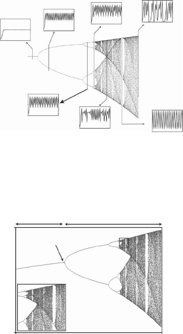
Figure 6.3 Depiction of the bifurcation diagram of the logistic equation after 10,000 iterations, x

, of the

recursive equation x

t+1

= ax

(1 − x

) for each value of a in relation to time series x

obtained for increasing

values of a; a = 2.00 (A), a = 3.261205 (B), a = 3.511687 (C), a = 3.57494 (D), a = 3.683735 (E), a = 3.828427

(F), a = 4.00 (G). The initiating value x

is set to x

= 0.05. (The bifurcation diagram was created with the

freeware Fractint of the Stone Soup Group.)

Unstability

Stability

1.9

3.9

a = 3

Chaotic region

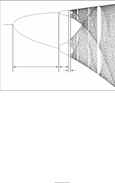
Figure 6.4 Depiction of the bifurcation diagram of the logistic equation after 10,000 iterations, x

, of the

recursive equation x

t+1

= ax

(1 − x

) for each value of a. The initiating value x

is set to x

= 0.05. Upon magni-

cation of a chaotic region (box) self-similar areas appear (inset). (The bifurcation diagram was created with

the freeware Fractint of the Stone Soup Group.)

2782.indb 204 9/11/09 12:12:48 PM

Fractal-Related Concepts: Some Clariﬁcations 205

6.1.2 FE i g E n b a u m un i v E r s a l nu m b E r s

As stressed above, the intervals between bifurcations decrease as a increases. Feigenbaum (1979)

recognized a universal pattern in the bifurcation events of a range of nonlinear dynamical equations

and characterized by the so-called Feigenbaum bifurcation constant d as (Figure 6.5):

−

(6.4)

For the logistic map (Figure 6.3), the Feigenbaum constant d has been estimated by Briggs (1991) to

84 decimal places and Briggs (1997) to 576 decimal places.

6.1.3 aT T r a c T o r s

The evolution of a dynamic system through time can be observed by tracing the instantaneous

values of n-state variables in n-dimensional space, the phase-space. A system in a steady state

will appear as a point in phase-space (that is, a stable equilibrium), while a stable oscillator traces

a closed loop through phase-space (that is, a stable limit cycle). The point and the closed loop are

both attractors for their respective systems; the systems develop toward those states regardless of a

range of boundary conditions and perturbations. The stable equilibrium and the stable limit cycles

are classical examples of attractors. A forced and damped oscillator (for example, a magnetically

driven pendulum with friction) may be represented in a 2D phase-space by its instantaneous angular

deection and speed (the two-state variables). An overdamped oscillator will spiral toward a point

attractor as it grinds to a halt, while under a range of forcing–damping ratios, the oscillating system

will trace out a closed loop in phase-space. However, this nonlinear system also exhibits chaotic

Figure 6.5 First set of three successive values of the driving parameter a of the logistic equation bifurcation

diagram used to estimate the Feigenbaum number d. (The bifurcation diagram was created with the freeware

Fractint of the Stone Soup Group.)

2782.indb 205 9/11/09 12:12:52 PM

206 Fractals and Multifractals in Ecology and Aquatic Science

behavior under the right conditions, and it traces as a fractal in phase-space. This fractal is an attrac-

tor for the system in phase-space, termed a strange attractor. After introducing the Packard-Takens

method used to visualize attractors (Section 6.1.3.1), these concepts are illustrated on the basis of

the phase-space signatures of purely deterministic signals (Section 6.1.3.2), random signals (Section

6.1.3.3), and chaotic signals (Section 6.1.3.4).

6.1.3.1 Visualizing attractors: Packard-takens method

Dissipative dynamical systems that exhibit chaotic behavior often have a strange attractor in phase-

space (Grassberger and Procaccia 1983). It is, for instance, the case for the movements of atmo-

spheric ows, which produce a specic phase-space trajectory now widely known as the Lorentz

attractor (Lorenz 1963). More precisely, a strange attractor has orbits that lie within a dened region

of phase-space but the orbits never intersect and never follow the same trajectory twice.

The phase-space attractor of a system is then a map of the changing conditions in the system;

each point on the attractor is a summary of all the variables affecting the system at a moment in

time. As the system evolves, changes in the variables result in a different location of the point

in phase-space. The points in phase-space trace a trajectory that summarizes the changes of the

system. Three-dimensional phase-space diagrams of the attractor describing the time series were

produced using the “time delay” method (Packard et al. 1980; Takens 1981). In practice, a one-

dimensional time series, and thus all the factors affecting it, can be represented by the trajectory of

points in three-dimensional phase-space. The attractor is created by plotting each value as a func-

tion of its preceding value, or in other words, from the plot of x (t + 1) vs. x(t), where x is the actual

value and t is the index of the point. Note that an attractor with a regular shape will also emerge in

plots using x (t + 2) or x (t + 3), for example, or x (t + n), with many n. This procedure is repeated for

each successive point in the time series and the resultant points are connected producing the phase-

space trajectory.

6.1.3.1.1 Periodic Attractors

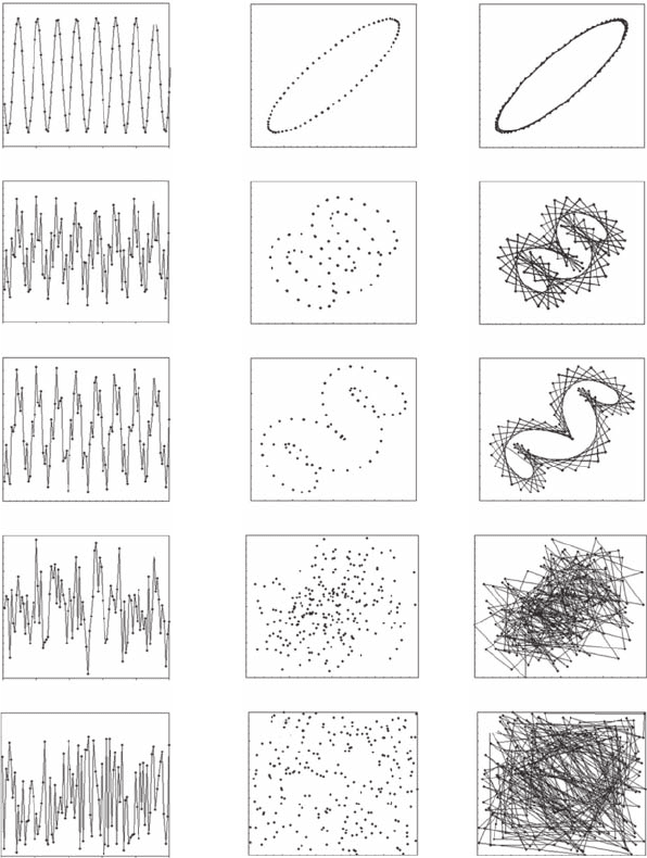
Consider a periodic function Y

with a single frequency, Y

= 0.4 sin (100t), where t is time. The

periodicity of Y

is obvious in the raw data (Figure 6.6A) and results in a stable orbit in phase-

space (Figure 6.6B,C). In contrast, in the case of a function without periodicity (that is, Y

= 0.4t + 0.4

and Y

= 0.4t

), the phase-space signature will consistently be a straight line (not shown). Now

consider a periodic function with two characteristic frequencies (Figure 6.6D), Y

= 0.4 sin (100t) +

0.4 sin (400t). An attractor with a regular shape will appear in phase-space using Y

t+n

, with any n

(Figure 6.6E,F). When the periodic function becomes more elaborate (Figure 6.6G), for example,

= 0.2 sin (20t) + 0.3 sin (100t) + 0.4 sin (400t), a clear attractor may still emerge depending on

the nature of the sine waves (Figure 6.6H,I), and may eventually need to be analyzed in more than

three dimensions to show any regularity.

6.1.3.1.2 Random Attractors

When a random noise is added to an otherwise periodic relationship (Figure 6.6J), the characteristic

shape of the attractors becomes very difcult to discern (Figure 6.6K,I). The phase-space portrait of

a random distribution (Figure 6.6M), in turn, does not exhibit any specic signature with simulated

points lling more or less the whole space evenly (Figure 6.6N,O).

6.1.3.1.3 Chaotic Attractors

Three of the most well-known and studied dynamical systems are briey presented hereafter, the

Hénon attractor and the Rössler and Lorenz attractors.

2782.indb 206 9/11/09 12:12:53 PM

Fractal-Related Concepts: Some Clariﬁcations 207

The Hénon attractor is dened by a recursive equation, H(x,

y) = (y + 1 − ax

, bx), where a and

b are adjustable parameters. An orbit, or trajectory, of the system consists of a starting point (x

, y

)

and its iterated images:

t+1

, y

t+1

) = (y

+ 1 − ax

, bx

) (6.5)

for k = 0, 1, … n. As previously discussed for the logistic equation, the dynamics of Equation (6.5)

strongly rely on the choice of the constants a and b. For a range of values for a and b, most orbits

0.5

0.3

0.1

–0.1

–0.3

–0.5

1.2

0.6

0.0

–0.6

–1.2

1.0

0.5

0.0

–0.5

–1.0

2.0

1.0

0.0

–1.0

–2.0

1.2

1.0

0.8

0.6

0.4

0.2

0.0

Time

02040 60 80 100

020406080 100

02040 60 80 100

020406080 100

t+1

0.5

0.3

0.1

–0.1

–0.3

–0.5

1.2

0.6

0.0

–0.6

–1.2

1.0

0.5

0.0

–0.5

–1.0

–1

–2

1.0

0.8

0.6

0.4

0.2

0.0

–0.5 –0.3 –0.1 0.1 0.3 0.5

–1.0 –0.5 0.0 0.5 1.0

–2 –1 012

0.0 0.2 0.4 0.6 1.00.8

–1.2 –0.6 0.0 0.6 1.2

0.5

0.3

0.1

–0.1

–0.3

–0.5

1.2

0.6

0.0

–0.6

–1.2

1.0

0.5

0.0

–0.5

–1.0

–1

–2

1.0

0.8

0.6

0.4

0.2

0.0

–0.5 –0.3 –0.1 0.1 0.3 0.5

–1.0 –0.5 0.0 0.5 1.0

–2 –1 012

0.0 0.2 0.4 0.6 1.00.8

–1.2 –0.6 0.0 0.6 1.2

Figure 6.6 Time series of different simulated signals Y

and the related phase-space portrait, Y

vs. Y

t+2

From top to bottom, a sine wave, Y

= 0.4sin(100t), a combination of two sine waves, Y(t) = 0.4 sin(100t) + 0.4

sin(400t), a combination of three sine signals Y(t) = 0.4 sin(100t) + 0.3 sin(100t) + 0.4 sin(400t), a combination

of the three sine signals and additive noise bounded between −1 and 1, and a random noise bounded between

−1 and 1.

2782.indb 207 9/11/09 12:12:57 PM

208 Fractals and Multifractals in Ecology and Aquatic Science

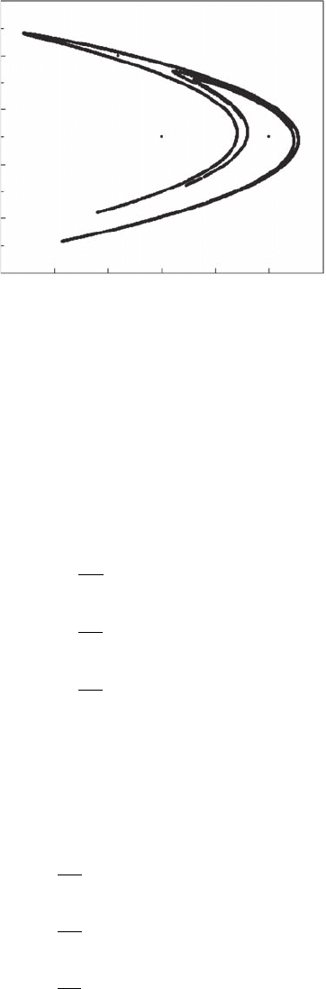
tend to a unique periodic cycle, while chaos dominates for a

1.4 and b

0.3 (Hénon 1976). The

resulting attractor is shown on a plot of y

vs. x

, for t = 10,000 (Figure 6.7).

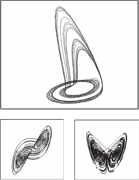
Both the Rössler and Lorenz attractors differ from the recursive logistic and Hénon equations as

they basically emerge from two systems of differential equations. Rössler’s system of differential

equations is (Rössler 1976):

xay

bxzcz

tt t

=− −

=+ −

()

(6.6)

The resulting attractor is shown in Figure 6.8A for a = 0.2, b = 0.2, and c = 5.7. Although the Rössler

system was articially designed to create a model for a strange attractor, the Lorenz model was

initially developed to simulate a global weather system (Lorenz 1963):

yRxyxy

Bz x

tttt

=− +

=− −−

=− +

σσ

(6.7)

where s, B, and R are the weather system parameters, xed at s = 10, B = 8/3, and R = 28. The cor-

responding attractor is shown in Figure 6.8B.

0.5

0.3

0.1

–0.1

–0.3

–0.5

–1.5 –1.0 –0.5 0.0

0.5 1.51.0

Figure 6.7 Phase-space portrait of the Hénon attractor. 10,000 points computed from Equation (6.5) with

, x

) = (0, 0), a = 1.4 and b = 0.3.

2782.indb 208 9/11/09 12:13:00 PM

Fractal-Related Concepts: Some Clariﬁcations 209

6.1.3.2 quantifying attractors: diagnostic methods for deterministic chaos

In the following, our data sets are regarded as nite sets of time observations, x(t), taken at regular

intervals:

X(t) = {x(1), x(2), …, x(n)} (6.8)

where n is the total number of observations in each set. The time length of any observed period, T,

is related to n as:

T = nΔt (6.9)

More specically, the three methods presented here—the Packard-Takens (PT) method (see

Section 6.1.3.1), Lyapunov exponents estimates (Wolf et al. 1985), and the correlation integral

method (Grassberger and Procaccia 1983)—are based on the assumption that the dynamics of any

underlying dynamical systems can be described in some multidimensional phase-space from the

knowledge of the time series of a single observation x(t) by constructing E-dimensional vectors

dened by:



Xt xt xt xt D

() ((), (),,(( )))=− −−τ 1

(6.10)

Figure 6.8 Three-dimensional phase-space portrait (x

, y

, z

) of the Rössler attractor (A) and two-

dimensional phase-space portraits (x

, y

) (B) and (x

, z

) (C) of the Lorenz attractor, shown for 5000 iterations.

2782.indb 209 9/11/09 12:13:09 PM

210 Fractals and Multifractals in Ecology and Aquatic Science

where D

is the embedding dimension (that is, the dimension of the vectors), and t is the lag (that is,

the number of data points separating each of the vector’s elements). For D

= 3 and t = 1, the vector



Xt()

consists of x(t) and the D

− 1 immediately preceding points of the time series; that is, the set

of vectors

{(), (),,()}







XX Xn34

is denoted as:

{( (),(), (),(((), (),()), ,((xxxxxx x321432 ((),( ), (( ))}nxnxn−−12

In the above case, the delay time t must be chosen so that it results in points that are not cor-

related to previously plotted points. Thus, a rst choice of t should be in terms of the decorrelation

time of the time series (Tsonis et al. 1993). A straightforward procedure is to consider the decorrela-

tion time equal to the lag at which the autocorrelation function for the rst time attains the value of

zero. Also note that no averaging or ltering should be employed since such data manipulations can

obscure the presence of chaos (Ellner 1992).

6.1.3.2.1 Largest Lyapunov Exponents

The limits of predictability are set by how fast the trajectories diverge from nearby initial condi-

tions. This feature is quantied by Lyapunov exponents, which are the average exponential rates

of divergence or convergence of nearby orbits in phase-space. Any system containing at least one

positive Lyapunov exponent is dened to be chaotic, with the magnitude of the exponent reecting

the time scale at which the system dynamics become unpredictable. In other words, the larger the

positive exponent, the more chaotic the system and the shorter the time scale of system predictabil-

ity (Wolf et al. 1985).

To dene the Lyapunov exponents, imagine an innitesimal hypersphere of initial condi-

tions in the n-dimensional phase-space. There is one Lyapunov exponent for each degree of

freedom of the system. We observe the evolution of the hypersphere as time progresses. The

hypersphere will be deformed into a hyperellipsoid because of the evolution of the system.

Then the ith Lyapunov exponent can be dened in terms of the length of the ith principal axis,

, of the ellipsoid as:

→

limln

()

∞

(6.11)

where the l

are ordered from largest to smallest in an algebraic sense (Wolf et al. 1985; Mundt

et al. 1991). A minimum condition for chaos is that the largest Lyapunov exponent (LLE), l

is positive.

In practice, the algorithm developed by Wolf et al. (1985) is recommended to estimate the larg-

est Lyapunov exponent, l

, from a time series, since it uses a relatively simple procedure and has

been demonstrated to be robust over a large range of input parameters and relatively accurate for

small, noisy data sets (Mundt et al. 1991). The delay time t should be chosen as the decorrelation

time of the time series, as previously mentioned.

6.1.3.2.2 Correlation Integral

Although the LLE is used to estimate the limits of predictability of a given time series, the comple-

mentary correlation integral (CI) algorithm is devoted to the quantitative characterization of the

attractor of the series. In particular, this method can be regarded as a generalization of the correla-

tion dimension described in Section 3.2.6. As demonstrated by Takens (1981), an attractor topologi-

cally equivalent to the attractor of the system producing the data is obtained for every value of t and

for D

sufciently greater than the fractal dimension, that is, D

≥ (2D + 1).

2782.indb 210 9/11/09 12:13:12 PM

Fractal-Related Concepts: Some Clariﬁcations 211

From the new multidimensional time series dened by Equation (6.10), the correlation integral

(Grassberger and Procaccia 1983) is dened as:

rXX

() lim=−−

(

)

→

=+=

∑∑

∞



(6.12)

where N is the number of distinct pairs in the embedding space,



−

is the Euclidean distance

operator between the ith and jth sample, r is an arbitrary time called “lag time” (distance between

vectors), and q(x) is the Heaviside function, dened as follows:

θξ

()=

≥











for<0

for0

(6.13)

The correlation integral C(r) represents the probability that the distance between a pair of randomly

chosen points on the D

-dimensional reconstruction will be less than a distance r apart (Grassberger

and Procaccia 1983). In the case of random processes, the phase-space trajectory is directly linked

to the volume of the considered D

-dimensional space as:

C(r) ∝

r→0

(6.14)

while for an attractor, the phase-space trajectory is more compact and the correlation integral is then

characterized by the following scaling properties:

C(r) ∝

r→0

(6.15)

where the exponent v is the correlation exponent (or correlation dimension); it can be estimated as

the slope of the log-log plot of C(r) vs. r, using a simple least-squares method.

For chaotic data, v will approach a constant value as the embedding dimension E is increased.

That constant value is an estimate of the correlation dimension that measures the local structure of

the strange attractor. The dimension v of the strange attractor indicates at least how many variables

are necessary to describe evolution in time. For instance, v = 2.5 indicates that a given time series

can be described by a system equation containing three independent variables.

6.1.3.2.3 Nonlinear Forecasting: Nearest-Neighbor Algorithm

Based on various prediction theories (Lorenz 1963; Tong and Lim 1980; Priestley 1980; Farmer

and Sidorowich 1989), this method was initially developed for (1) making short-term predic-

tions about the trajectories of chaotic dynamical systems, and (2) distinguishing between the

complexity of natural dynamical systems where deterministic dynamics can lead to chaotic tra-

jectories and the uctuations intrinsically related to the sampling and measurement processes

(Sugihara and May 1990b; Sugihara et al. 1990; Sugihara 1994). A direct consequence of the

sensitive dependence on initial conditions of a chaotic system is that prediction will become

exponentially less accurate as one attempts to predict further ahead. The nearest-neighbor (NN)

algorithm quanties this prediction accuracy as a function of the distance into the future that

they are made. Specically, the D

-dimensional vectors introduced in Equation (6.10), that is,



Xt xt xt xt D

() ((), (),,(( )))=− −−τ 1

, are used to calculate the distance between



Xt()

and the k

2782.indb 211 9/11/09 12:13:17 PM

212 Fractals and Multifractals in Ecology and Aquatic Science

nearest-neighbors vectors



Xt Xt xt xt xt D

ii ii iE

(),()((),( ), ,( ()))=−−−

ττ

, and the predicted value

of each x(t) is given as:

xt p

() ()+= +

∑

(6.16)

where p is the prediction distance, that is, the number of steps ahead that one is attempting to pre-

dict. The predicted values x(t + p) are then plotted against the actual values x(t), and the strength

of the predictions evaluated through their coefcient of correlation r. Practically, the rst half of a

given data set X(t), see Equation (6.8), is used to estimate x(t + p), which is then plotted against the

second half of X(t).

Two sets of information are subsequently derived from the coefcient of correlation r, and used

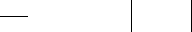
to classify the dynamics of the system under study. First, a plot of the coefcient of correlation r as

a function of the prediction time provides information on the deterministic vs. chaotic nature of the

system. For instance, purely deterministic (that is, nonchaotic) processes will return consistently

high values of r whatever the prediction distance (Figure 6.9). In contrast, chaotic systems such as

the logistic equation in the regime where a > 3.5749 lead to an exponential decrease of r as prediction

time increases (Figure 6.9A). Note that the contamination of the logistic equation by external (white)

noise* decreases uniformly the predictability of nonchaotic systems, depending on the amplitude of

In which case, Equations (6.2) and (6.3), respectively, rewrite as x

t+1

= ax

(1 − x

) + e(t) and x

t+1

= ax

− ax

+ e(t).

1.0

0.8

0.6

0.4

0.2

0.0

5101520

1.0

0.8

0.6

0.4

0.2

0.0

0510 15 20

Figure 6.9 Nearest-neighbor technique applied to the logistic equation (see Equations 6.2 and 6.3). Top

panel: a = 2.5 (A: dashed line), a = 3.5 (A: open dots) and a = 4.0 (thick black curve), a = 4.0 with external noise

, e(t) = ±0.005 (thick gray curve), and a = 4.0 with external noise e

, e(t) = ±0.05, (thin black curve). Bottom

panel: a = 3.5 with external noise e

, e(t) = ±0.005, (black line) and e(t) = ±0.05, (gray line) and a = 3.5 with

process noise e

, e(t) = ±0.005 (open triangles) and e(t) = ±0.05 (open diamonds), and a = 2.5 with external

noise e

, e(t) = ±0.005 (dashed line) and e(t) = ±0.05 (not shown, indistinguishable from r = 0) and a = 25 with

process noise e

, e(t) = ±0.005 (dashed thick gray curve) and e(t) = ±0.05 (black dots).

2782.indb 212 9/11/09 12:13:21 PM

Fractal-Related Concepts: Some Clariﬁcations 213

the noise (Figure 6.9B). In contrast, noise-contaminated chaotic systems will steepen the exponen-

tial decay of predictability (Figure 6.9A). Internal noise,* in turn, leads to a nonexponential decay

in the predictability of a nonchaotic system (Figure 6.9B), unless the magnitude of the noise is suf-

cient to drive the system into the unstable chaotic regime (Sugihara 1994) (Figure 6.9B). Second,

the shape of a plot of r as a function of the embedding dimension D

informs on the dimensionality

of the system; chaotic systems show optimal predictability for low embedding dimensions, while

random processes exhibit increasing predictability at higher embedding dimensions.

6.1.3.3 case study: Plankton distribution in turbulent coastal waters

6.1.3.3.1 Ecological Framework

A range of empirical and theoretical studies have demonstrated that fully developed turbulence is

rather characterized by its multifractal properties (that is, high-order stochasticity and high dimen-

sionality); see, for example, Frisch (1996) and references therein. Ruelle and Takens (1971) also

showed that near the transition to turbulence, the many degrees of freedom of turbulence are cou-

pled coherently and lead to an enormous reduction in dimension (that is, low-order deterministic

chaos emerges). It is then likely that in aquatic environments characterized by uctuating turbu-

lent intensities (for example, shallow coastal and estuarine regions), the structure of both physical

(temperature and salinity) and biological (phytoplankton biomass) parameters vary considerably.

In other words, the dimensionality and predictability of a system might be related to the turbulent

conditions.

Specically, such transitions between low-order deterministic chaos and high-order stochas-

ticity may be observed in the tidally mixed waters of the eastern English Channel (Figure 4.8),

where turbulence intensities may vary by more than two orders of magnitude over one tidal cycle

(Seuront 2005b; Seuront et al. 2002) and are generally thought to drive phytoplankton biomass

variability (Seuront et al. 1996a, 1996b, 1999). Herein, the goal of this case study is, rst, to nd

out whether time series of physical (temperature and salinity) and biological (phytoplankton bio-

mass) parameters recorded in tidally mixed waters are chaotic or not, and second, to investigate

the potential effects of differential tidal forcing on the chaotic or stochastic nature of the variables

in question.

6.1.3.3.2 Experimental Procedures and Data Analysis

The sampling experiment was conducted during 60 hours (that is, ve tidal cycles) in a period of

spring tide, from March 28 to 30, 1998, at an anchor station located in the coastal waters of the

eastern English Channel (50°47′300 N, 1°33′500 E) (Figure 4.8). The tidal range in this system

is one of the largest in the world, ranging from 3 to 9 m, and the water column is believed to be

fully homogenized by tide-generated turbulent mixing. Temperature, salinity, and in vivo uores-

cence were simultaneously recorded at 2 Hz from a single depth (5 m) with a SBE 25 Sealogger

CTD (conductivity-temperature-depth) probe, and a Sea Tech uorometer, respectively. Every hour,

samples of water were taken at 5 meters depth to estimate chlorophyll a concentrations, which

appear signicantly correlated with in vivo uorescence (Kendall’s t = 0.778, p < 0.01). In the fol-

lowing, the latter parameter will then be regarded as a direct estimate of phytoplankton biomass.

To investigate the potential effect of varying turbulent forcings on the local structure of physical and

biological parameters, the data analyzed here consist of 24 time series (labeled from S1 to S24) of

1 hour duration (7200 data points), resampled from the original data set in order to be representative

of the different conditions of tidal current speed and direction, taken every 10 minutes, from the

sampling depth (Table 6.1).

Time-series analysis requires the assumption of at least reduced stationarity; that is, the mean

and the variance of a time series depend only on its length and not on the absolute time (Legendre

Now Equations (6.2) and (6.3), respectively, rewrite as x

t+1

= a(x

+ e(t))(1 − (x

+ e(t)) and x

t+1

= a(x

+ e(t)) − a (x

+ e(t))

2782.indb 213 9/11/09 12:13:22 PM