Sandau R. Digital Airborne Camera: Introduction and Technology
Подождите немного. Документ загружается.


4.8 Flight Management System 233
properly. The lines flown had to be tediously plotted on a map when the flight
report was drawn up following the flight mission. Thanks to GPS, high-performance
receivers and related computer hardware and software, these operations are consid-
erably easier today. Flight management systems (FMSs) for supporting navigation
and determining position are the key to successful and cost-effective surveying
flights. A modern FMS combines the advantages of a GPS-based surveying flight
system with those of a sensor control system that is largely automated and that
supports continuous data flow from planning to data processing (Fig. 4.8-1).
Flight evaluation
Quality control
Flight
planning
Flight
execution
Data
processing
Fig. 4.8-1 Processing chain
This section deals mainly with sensor and FMS software. For the sake of clarity
in delineating the functions and interfaces, we first deal with flight planning and
flight evaluation. This will be followed by a more detailed description of sensor
control and flight execution. Data processing is dealt with in Chapter 6.
4.8.1 Flight Planning
Flight planning is the first step in the processing chain and is normally done at the
office. If planning errors are noticed when the aircraft is already in the air, how-
ever, plans may have to be corrected during flight. A plan lays down the flight lines
required to cover the project area according to the specifications. It can also be used
for optimising the flight course to provide the pilot with flight guidance support.
In practice, the task for a flight project may be formulated as follows: “Map the
city centre area in colour using a ground resolution of 10 cm and a lateral overlap
of 60%.” When planning this flight, the outline of the specified area is scanned as
a polygon on existing maps. In the case of paper maps, a digitiser is used for this
purpose and, in the case of digital maps, it is done directly on the computer screen.
Taking into account the sensor geometry and the specified boundary conditions such
as coordinate system, overlap and preferred flight direction, the flight lines are opti-
mised and, depending on the sensor type, the camera triggering or start and stop
points plotted. If required, additional flight lines, individual images or waypoints
needed for geometric stabilisation of the processed data, for a desired flight path
or for other purposes can be added. The completed plan is exported as a file to be
used for executing the flight. Modern planning software has an interactive graphi-
cal user interface, which instantly displays the result when parameters are changed.
Moreover, high-performance flight planning software supports planning in various
coordinate systems and over multiple map zones and enables a digital terrain model
(DTM) to be used for flight plan optimisation. An integrated system and a contin-
uous processing chain make it possible to establish the configuration of the map
system even when plotting the flight plan.
234 4 Structure of a Digital Airborne Camera
4.8.2 Flight Evaluation
It is important to have quality control and clarity about the project status after each
step in the process. For instance, after a flight, the user wants to have a comparison
between the planned data and the flight data. Imaging material is passed on to the
next processing step only after the operator has checked to see if all data has been
captured as specified, i.e., the software must be able to evaluate flight plan data
against the actual flight data. But to be able to make a detailed analysis after a flight,
all requisite information, such as GPS positions, camera triggering or start and stop
points, additional data generated by the operator (for example, clouds in the image),
camera status and error messages, needs to be recorded by the FMS during the
flight. After the flight, this data is transferred from the flight system to the office for
evaluation.
4.8.3 Flight Execution
After flight planning, the next stage in the processing chain is flight execution, in
which the flight plans are copied from the office to the flight system. As explained
above, numerous factors impose constraints on the flight mission. In general, the
execution of a flight involves a great deal of work and is very cost-intensive. A flight
mission must therefore be carried out as efficiently as possible. This is facilitated by
a camera system that is largely automated. Based on the flight plan data, it operates
almost without user interaction, automatically recognizes errors and informs the
operator about the status of the system. For a flight mission to be successful, it is
necessary to have an optimised and correct flight plan.
During the flight, the flight management system (FMS) interprets the flight plan
selected and performs the following principal tasks:
(1) Flight guidance along all lines of the flight plan, including quality control and
autotracking of the project status
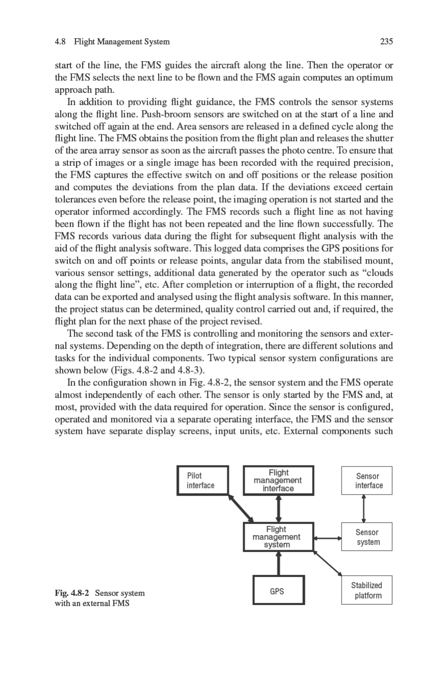
(2) Control and monitoring of sensors and external systems in accordance with the
flight plan data.
At the start of the flight, the operator selects a flight plan and the next line to be
flown. Based on the current position, the FMS computes an optimum flight path to
the start of this line, taking into account the definable flight parameters. The current
position required for this purpose is provided by the GPS. The coordinates of the
start of the line are provided by the flight plan. The optimum flight path is displayed
for the operator and the pilot. Most systems have display screens that are optimised
to meet the requirements of the operator and the pilot. As a rule, the pilot flies along
the proposed flight path. The proposed flight path is not binding, however, and there
is a number of reasons for which the pilot may choose to deviate from the proposed
flight path. If this occurs and a definable tolerance is exceeded, the system computes
a new approach path based on the current position. After the aircraft reaches the
4.8 Flight Management System 237
small separate display screen is usually provided to support the pilot with graphic
and numeric navigation data to enable him to follow the flight pattern laid down
in the plan. Deviations from the target course are displayed and the optimum flight
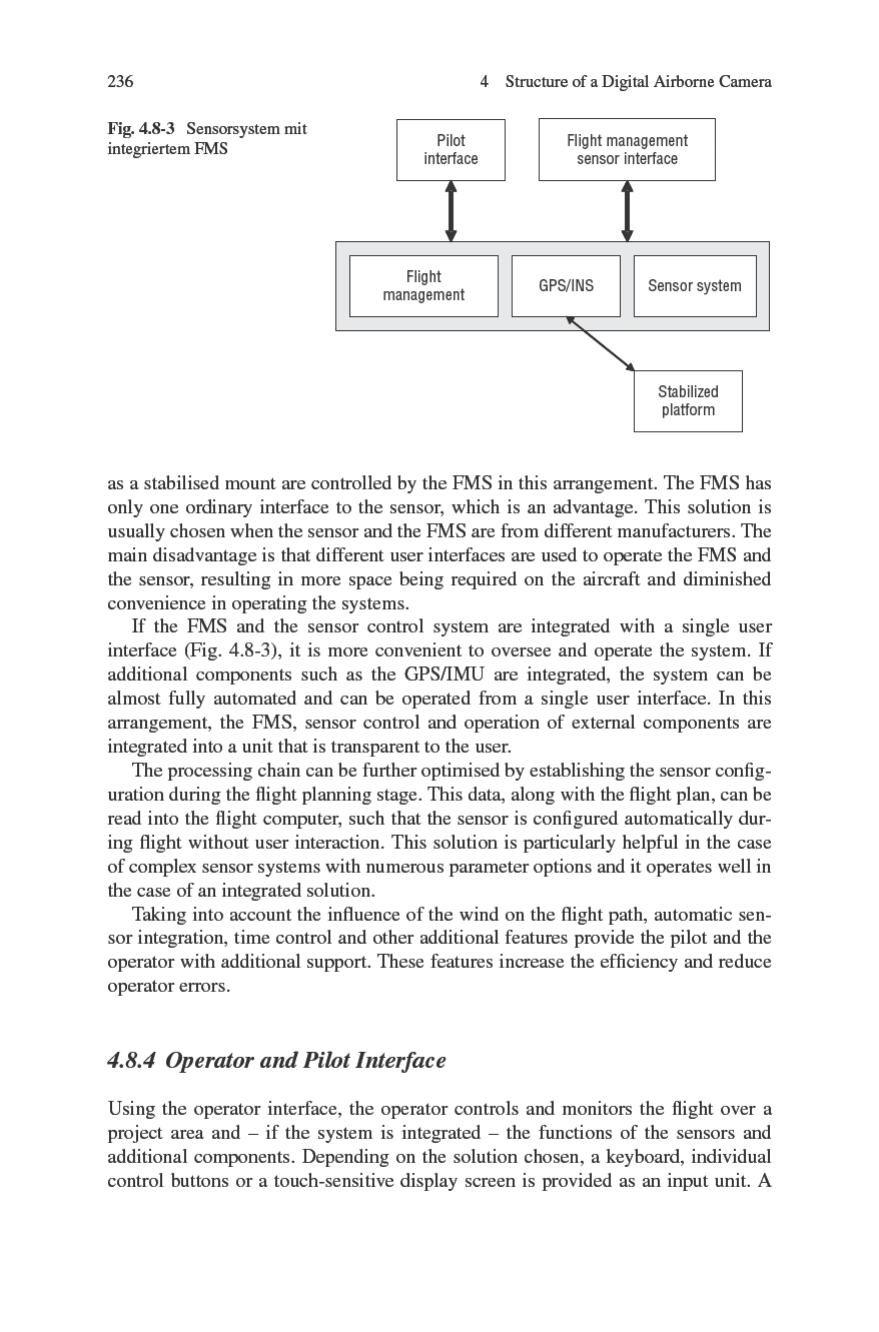
path suggested. In the case of an integrated system, it is even possible to control
the entire system via the pilot interface. This enables the pilot to carry out the flight
mission on his own. To meet the different data requirements of the camera operator
and the pilot, it is advisable to have the screen content and the information tailored
to their particular requirements and displayed independently on the operator and
pilot interfaces. Only few systems support this, however, and most systems provide
the operator and the pilot with the same information, which makes it necessary for
them to coordinate their work during the flight accordingly.
To conclude this section, two views of the Leica FCMS are shown below
(Figs. 4.8-4 and 4.8-5). These show what an integrated user interface can look like
and the options available.
4.8.5 Operator Concept
The FCMS is operated via a touch-sensitive screen. A keyboard is not required.
Whenever possible, graphic elements are used and text is used only if necessary.
Ten context-sensitive pictogram fields are available as control elements.
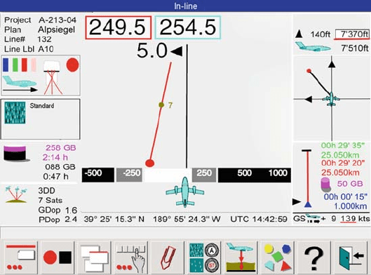
In the navigation view (Fig. 4.8-4), the control fields down the left-hand side are
as follows (top to bottom): general project information; sensor status; image class;
mass memory status; and GPS status. The control fields down the right-hand side
are as follows (top to bottom): flight altitude; bearing; line status; and flight speed
Fig. 4.8-4 Navigation view “on the line” in the Leica FCMS
238 4 Structure of a Digital Airborne Camera
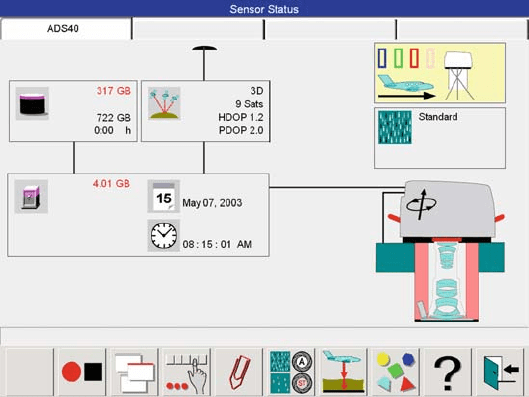
Fig. 4.8-5 Sensor status as seen on the Leica FCMS
over ground. The information in the centre of the image comprises: graphics display
for navigating along the flight line, position and UTC time. The bottom part of the
view consists of a status line and pictogram fields for user commands.
In the sensor status view (Fig. 4.8-5), the control fields down the left-hand side
are as follows (top to bottom): mass memory status; GPS status; computer memory
status; time information; and date. The control fields down the right-hand side are
as follows (top to bottom): sensor status; image class; and hardware status of sensor
head. The bottom part of the view consists of a status line and pictogram fields for
user commands.
4.9 System for Measurement of Position and Attitude
4.9.1 GPS/IMU System in Operational Use
For the operational use of GPS/IMU systems for measuring positioning and attitude,
the definition of system performance and requirements is elementary. As already
indicated in the introductory part of Section 2.10, system choice depends on fac-
tors such as the following. Are the integrated GPS/IMU systems used as standalone
components for the direct georeferencing of airborne sensors, or is the exterior
orientation directly measured by GPS/IMU further refined in a process of aerial
triangulation? As an extreme example, the GPS/IMU exterior orientations may be
used only as initial approximations for the aerial triangulation. What are the final
required accuracies for position and attitude? Are the GPS/IMU sensors used in very
high dynamic or low dynamic environments? Is GPS update information available
4.9 System for Measurement of Position and Attitude 239
almost continuously or are there long sequences which have to be bridged because
GPS data is not available? Such scenarios often occur in land applications owing
to satellite blocking in built-up areas. Is alternative update information available
besides GPS? Is there a need for real-time navigation? What reliability in naviga-
tion has to be guaranteed throughout the mission? All these factors lead to solutions
that are application dependent, so within this context general recommendations are
difficult.
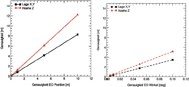
The following discussion covers the influence of variations in the accuracy of
the parameters of exterior orientation (for example, from GPS/IMU systems) on the
determination of object points. As can be seen from Fig. 4.9-1, variations in exterior
orientation certainly affect the performance. The results depicted in the figure are
from simulations based on the following input values: stereo pair of images, stan-
dard 60% forward overlap, image format 23 × 23 cm
2
, camera focal length 15 cm
(wide-angle optics), flying height above ground 2,000 m, image scale 1:13,000. The
true image coordinates of 12 homologous points within the stereo model are overlaid
with random noise of standard deviation 2 μm. This noise represents the accuracy of
standard image measurements. The resulting object coordinates are obtained from
direct georeferencing based on the simulated exterior orientation elements. Finally,
the coordinates of object points are compared to their reference values. Figure 4.9-1
shows how object point accuracy depends on variations in the quality of exterior
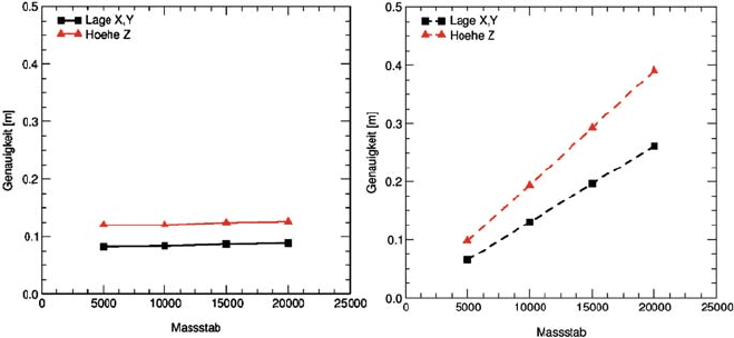
orientation, whereas Fig. 4.9-2 is obtained from exterior orientations with fixed
accuracy (i.e. position σ
X,Y, Z
= 0,1 m, attitude σ
ω,φ,κ
= 0.005) and depicts the
influence of variations in flying height and image scale. Again the final accuracy
of object point determination is illustrated. As in the case of the first simulation,
the image coordinates are overlaid with 2 μm noise. All other parameters remain
unchanged from the first simulation.
As expected, the quality of exterior orientation has a direct influence on the accu-
racy of point determination. In all cases the object point performance is linearly
dependent on position and attitude accuracy as well as flying height and image
Fig. 4.9-1 Influence of variations in the accuracy of positioning ( left) and attitude (right) on object
point determination from direct georeferencing
240 4 Structure of a Digital Airborne Camera
Fig. 4.9-2 Influence of variations in image scale and flying height on object point determination
from direct georeferencing, assuming constant accuracy of positioning (left) and attitude (right)
scale. Assuming positional errors in exterior orientation of about σ
X,Y, Z
= 5m in
all components, the accuracy finally obtained in object space is around 5 m (mean).
The performance in the height component is worse due to the specific geometry of
image ray intersection. Similar behaviour can be seen if erroneous attitude informa-
tion is assumed. With an orientation error of σ
ω,φ,κ
= 0.05
◦
the resulting error in
object space is about 1.7 and 2.6 m for horizontal and vertical components respec-
tively. This error budget can also be estimated by using the well known equation
h
g
·tan (σ
ω,φ,κ
), where h
g
describes the flying height above ground. The overall influ-
ence caused by both position and attitude errors is derived from the two individual
errors by means of the rules of error propagation.
If the accuracy of the attitude values remains constant (σ
ω,φ,κ
= 0.05
◦
), the
performance in object space decreases linearly with increasing flying height, which
corresponds to a decrease in image scale, assuming that the camera constant remains
unchanged. On the other hand, the influence of positioning errors in exterior orien-
tation is almost unaffected by flying height and image scale, but remains constant
for the range of image scales covered. Only a very small decrease in accuracy is
visible for smaller image scales. This is due to the overlaid noise in image coordi-
nate measurements, which has slightly more influence in the case of smaller image
scales acquired from higher flying heights: image space errors have more effect
in object space if small scale imagery is considered. If one directly compares the
influence of positioning and attitude errors on the overall error budget in object
space (Fig. 4.9-2), the influence of attitude errors dominates for flying heights above
approximately 1,000 m (corresponding image scale 1:6,500). Note that this thresh-
old holds for the chosen simulation parameters only. For very large scale flights from
low flying heights, the influence on positioning errors is the limiting factor in direct
georeferencing. For small scale imagery from high altitudes, the attitude perfor-
mance is the dominating factor with respect to the quality of direct georeferencing.

4.9 System for Measurement of Position and Attitude 241
Depending on the desired applications, the main focus has to be on higher posi-
tioning performance or alternatively higher quality in attitude determination. This
ultimately defines the quality requirements for GPS/IMU exterior orientations (see
Fig. 4.9-1), as well as the approaches taken for GPS/IMU processing (i.e. real-time,
post-processing, GPS processing [Table 2.10-1)].
For digital camera systems, the maximum tolerable error in object space is lim-
ited by the sensor’s ground sampling distance (GSD). Assuming that the smallest
object to be identified in the images has to be at least the size of one object pixel,
the required accuracy of object point determination also has to be in the range of
one object pixel or better. From this the following equation can be found:
h
g
= c ·m
b
= c ·
GSD
pix
=
c
pix
·GSD = k ·GSD. (4.9-1)
The resulting flying height above ground h
g
is a function of camera f ocal length
c and sensor pixel size pix. The k factor is obtained from the quotient of these. Its
reciprocal value
1
k
=
pix
c
is known as the instantaneous field of view (IFOV) of the
sensor. Equation (4.9-1) also shows that in the case of digital imaging the GSD plays
a similar role to image scale in data acquisition from the former analogue imagery.
Integrated GPS/IMU systems used for the direct orientation of airborne sensors
are typically used in the following circumstances. The update information from GPS
is available throughout the whole mission flight. If any satellite blockages and signal
loss of lock are present, they appear mainly during flight turns. Sequences without
any GPS update information are relatively short. Within the remaining parts of the
trajectory, enough GPS data is available between two signal loss of lock events to
resolve the integer phase ambiguities reliably. This is mandatory in the case where
differential carrier phase processing is required and applied. Such considerations
are of importance in the case of decentralized GPS/IMU data processing. Here raw
GPS measurements (pseudo-range, doppler and phase observations) are not used
for update, but already processed GPS position and velocity data (so-called pseudo-
observations) are fed into the filter. This requires a minimum of four satellites to
provide update information. Alternatively, if the GPS/IMU processing is performed
within a centralized filtering approach, raw GPS observations are used as update
information. Thus updates are possible even within periods where less than four
satellites are available. Nevertheless, GPS/IMU systems used in airborne appli-
cations for direct sensor orientation are mostly based on the decentralized filter,
owing to the higher flexibility of decentralized filters if additional components are
integrated, i.e. updates from other sensors. This is different to centralized filters,
where major parts of the algorithm have to be redesigned for changes in system
configuration.
If such integrated GPS/IMU systems for measurement of position and attitude
are used in dynamic environments, a certain bandwidth and sampling rate have to
be achieved to describe the dynamics of the sensor’s movement sufficiently. Since
the high frequency parts of the dynamics are measured by the inertial sensors, the
IMU specifications are of major concern. Within Fig. 4.9-3 two different spectra
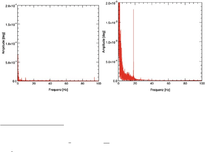
242 4 Structure of a Digital Airborne Camera
from inertial attitude determination are given for the same IMU chosen for this
example, in both static and airborne kinematic environments. The inertial data were
measured with 200 Hz frequency, thus frequencies up to 100 Hz are detectable. The
influence of the different system dynamics is obvious. Notice the different scaling
of the amplitude axis.
For the static environment almost no external vibrations are present. The frequen-
cies visible in the first spectrum are mostly due to the sensor-specific measurement
noise.
1
This situation is different for the same sensor if analysed in kinematic mode.
The frequency plot is obtained from data from a small portion of a flight, where the
aircraft was on a photogrammetric image strip. In contrast to the static spectrum,
higher amplitudes and additional lower frequencies <15 Hz are present, representing
the dynamics of this specific airborne environment. If the inertial sensor is rigidly
fixed to the aircraft’s body, this spectrum represents the movement of the aircraft.
Quite often, however, the IMU is fixed on a stabilized platform close to the imaging
sensor itself. In such cases the spectrum represents the dynamic environment of the
sensor. The kinematic spectrum in Fig. 4.9-3 shows a dominant peak around 18 Hz.
This reflects vibrations caused by the aircraft engines. In the higher part of the spec-
trum additional small frequency peaks are present, but with much lower amplitudes.
Such frequencies are negligible as long their amplitudes are smaller than the pixel
resolution of the sensor to be oriented. If one considers a digital camera with 10 ×
10 μm
2
pixel size in image space and a focal length of 10 cm, the resulting IFOV is
about 0.1 mrad (corresponding to 0.006
◦
). If such a camera is used in combination
Fig. 4.9-3 Spectral analysis of IMU attitudes (pitch angle) in static environment (left) and during
a photogrammetric flight (right)
1
The sensor-specific noise is dependent on the performance of the gyros and accelerometers. For
attitude sensors the performance of the IMU gyros is critical. The noise is given by the random
walk coefficient denoted in
◦
/
√
h
ˆ=60 ·
◦
/h/
√
Hz
. If this random walk coefficient is multiplied
by
√
t the accuracy of attitude determination after a certain time interval t[h] is estimated.