Roff D.A. Modeling Evolution: An Introduction to Numerical Methods

Подождите немного. Документ загружается.

> print(“Summary data for persistence times”);Data.Gens

[1] “Summary data for persistence times”

Min. 1st Qu. Median Mean 3rd Qu. Max.

1.00 6.00 13.00 19.09 25.00 100.00

Before discussing this output let us return to the summary objects. The summary

object in the present case contains six pieces of information: the minimum value,

the ﬁrst quantile, the median, the mean, the third quantile, and the maximum.

These components can be accessed separately: suppose, for example, we only

wanted the mean value of Npops, which is the fourth entry in Data.Npops: to

get this we simply use Data.Npops[4].

Returning to the above output: the mean population size is only 315.7, which is

far below the expected value of 250,556.6, though the maximum population size

is 1,570,0000, which is far above the expected population size. Unfortunately, the

summary function does not give the sample sizes and so it is not possible from this

information to assess how many populations persisted through the entire simula-

tion. To extract this information we can use the R function length, which gives

the number of elements in an object:

length(Pops.not.extinct) # number of populations that persisted

which gives 109: so out of 10,000 replications only 1.09% persisted for 100 gen-

erations.

Step 14: Further model analysis: more on lists

It is clear that the predicted population size from the deterministic model (model

1) does not match the result from the stochastic model with the same mean rate of

increase (model 2). To further illustrate the list construct let us statistically com-

pare the population sizes from model 2 with the size predicted by model 1. For

simplicity I shall use a single sample t-test, recognizing that the extreme skew in

the distribution makes such a test suspect (but this is for illustration of lists not

statistical rigor). This test is available in the statistics toolbox of MATLAB. The

R code, saving the output as an object called T.results,is

Data <- Npops-250556.6 # Subtract predicted value

T.results <- t.test(Data) # T test with null of zero

T.results # Print out results of t test

The result is

One Sample t-test

data: Data

t ¼1501.757, df ¼ 9999, p-value < 2.2e16

alternative hypothesis: true mean is not equal to 0

95 percent confidence interval:

250567.6 249914.3

sample estimates:

mean of x

250240.9

38 MODELING EVOLUTION

Obviously the difference is highly signiﬁcant, even given the skew in the data. The

object T.results consists of a list of items that can be accessed individually in a

number of ways. First, to determine what items are in the list we issue the code

names(T.results) # Names of the items in the object T.results

with the result

[1] “statistic” “parameter” “p.value” “conf.int” “estimate”

[6] “null.value” “alternative” “method” “data.name”

The estimate is located in position 5 and can be accessed in the following ways:

T.results[5]

T.results[[5]]

T.results$“estimate”

which give three slightly different outputs (but not different values):

> T.results[5]

$estimate

mean of x

250240.9

------------

> T.results[[5]]

mean of x

250240.9

------------

> T.results$estimate

mean of x

250240.9

------------

If one wishes to use the resulting variable the second two methods are preferred

since, for example, T.results[5]^2 results in the error message “Error in T.

results[5]^2 : non-numeric argument to binary operator”. If one wished

to convert the value to a simple numerical value and eliminate the accompanying

label “mean of x” use the function as.numeric, as in, for example,

a <- as.numeric(T.results$estimate)# Convert value to numeric

Step 15: An analytical aside: what is going on?

The present model results indicate that the arithmetic mean growth rate does not

appear to be a good index of population persistence in a temporally stochastic

environment. If this is the case then perhaps the arithmetic mean growth rate is

also not an appropriate measure of ﬁtness in a stochastic environment. Haldane

and Jayakar (1963) and Cohen (1966) showed that the appropriate measure is the

geometric rate of increase. The reason for this resides in the difference between

the geometric and arithmetic means (Lewontin and Cohen 1969). In our model

population size at time t is given by

OVERVIEW 39

tþ1

¼ N

...l

¼ N

i¼1

ð1:32Þ

We assumed that l

is a random, uncorrelated variable with mean



. The expected

population size at time t is then given by the product of the initial population

size, N

, times the expectation of the product l

...l

. Because the l’s are

uncorrelated, the expected value of the product is equal to the product of the

expected values, giving

EfN

g¼N

i¼1

g¼N

i¼1

Efl

g¼N



t ð1:33Þ

At ﬁrst glance the above result suggests that an appropriate measure of ﬁtness is



which is the arithmetic mean of the ﬁnite rates of increase (i.e., l



i¼1

) not the

geometric, which is given asl



¼ðP

i¼1

. However, the behavior of populations ina

temporally randomly varying environment has the curious property that the expec-

tation of populationsize willgrow without bound whenever



> 0 butthe probability

of extinction within a few generations can be virtually certain (Lewontin and Cohen

1969; Levins 1969; May 1971, 1973; Turelli 1977). This paradoxical behavior can be

illustrated with a simple example: suppose that l can take two values, 0 or 3, with

equal frequency. The expected value of l is (0 þ 3)/2 ¼ 1.5, and hence the expected

population size increases without bound as t increases. For example, starting from a

single female, after 10 generations E{N

} ¼ 1.50

¼ 57.7 but either N

¼ 59,049 or

¼0 and the probabilitythatthepopulation persists for the10 generationsis (0.5)

¼ 0.00098, a very small probability indeed! The geometric mean is always smaller

than the arithmetic and the two are related by the approximation Eðln lÞln l



(Lewontin and Cohen 1969), where E(lnl) is the geometric mean,



is the arithmetic

mean, and s

is the variance. Selection should operate to increase the arithmetic

mean and decrease its variance, which will increase the geometric mean.

Step 16: Adding spatial heterogeneity

The important conclusion from the model so far is that temporal heterogeneity

could be an important selective agent favoring particular types of life history. Our

impetus for this analysis was the hypothesis that migration is an important evolu-

tionary response to environmental heterogeneity. Thus the next step of the analysis

is to introduce spatial variation, initially keeping all subpopulations isolated.

1.4.4 Mathematical assumptions of model 3

1. The habitat is divided into a number of discrete patches.

2. Rates of increase are stochastically variable and uncorrelated among patches.

3. There is no migration of animals among patches.

There is no conceptual difference between this model and the previous model but

there are two avenues by which it could be programmed:

1. Each population is run over its entire simulation within the function as previ-

ously done, with the main program iterating over patches.

40 MODELING EVOLUTION

2. The function could compute the single generation change for all populations

and the function called iteratively for each generation of the simulation.

In the subsequent model we wish to introduce migration between habitats at

each generation which could not be done under the ﬁrst approach. Thus the

second approach is appropriate in this instance. The coding is a straightforward

extension of the previous approach with the following changes:

1. Within the POP function the number of random LAMBDA values generated is

equal to the number of patches, not the number of generations.

2. The mean population size (called Npop.Sizes) is followed, which is obtained

using the R and MATLAB function mean:

Npop.Sizes[Igen] < mean(Npop) # R code

Npop_Sizes(Igen) ¼ mean(Npop); % MATLAB code

where Npop is the vector of population sizes at generation Igen.

3. The simulation is stopped when either the maximum number of generations is

reached or the mean population size is zero (i.e., all populations are extinct).

4. In addition to mean population size the program also keeps track of the

number of extinct populations over time, N.e xtinc t[ Ig en] (another exam-

ple of matrix-wide comparison). The R and MATLAB codes are, respectively,

N.extinct[Igen] < length(Npop[Npop¼¼0]) # Store number of

extinct popns

N.extinct(Igen) ¼ length(Npop(Npop¼0)); % Store number of

extinct popns

The full coding in R is

rm(list=ls()) # Clear memory

POP <- function( MAX.Lambda, Npop, N.patches ) # Population

function

{

LAMBDA <- runif(N.patches, min¼0, max¼ MAX.Lambda)# Generate

lambdas

Npop <- Npop*LAMBDA # Generate new population size for all patches

Npop[Npop<1] <- 0 # Check for extinction

return (Npop) # Return the vector of new population sizes

} # End of function

#################### MAIN PROGRAM ####################

set.seed(100) # set seed

MAXGEN <- 100 # Set maximum number of generations

N.init <- 20 # Initial population size

MAX.LAMBDA <- 2.2 # Maximum value of lambda

N.patches <- 10 # Number of patches

Npop <- matrix(N.init, N.patches, 1) # Initialise populations

Npop.Sizes <- matrix(0,MAXGEN) # Pre-assign storage for

mean popn size

OVERVIEW 41

Npop.Sizes[1] <- mean(Npop) # Store first generation mean

popn size

N.extinct <- matrix(0,N.patches,1) # Storage for nos of

extinct popns

Igen <- 1 # Initialize generation counter

while ( Igen<MAXGEN && Npop.Sizes[Igen]>0) # Start while loop

{

Igen <- Igenþ1 # Increment generation

Npop <- POP(MAX.LAMBDA, Npop, N.patches) # New population sizes

Npop.Sizes[Igen] <- mean(Npop) # Store mean population size

N.extinct[Igen] <- length(Npop[Npop¼¼0]) # Store number of

extinct popns

} # End of while loop

par(mfcol¼c(1,2)) # Divide graphics page into two

# Plot Mean population size over generations and nos extinct per

generation

plot(seq(1, Igen), Npop.Sizes[1:Igen], xlab¼“Generation”,

ylab¼“Mean population size”, type¼“l”)

plot(seq(1, Igen), N.extinct[1:Igen], xlab¼“Generation”,

ylab¼“Mean population size”, type¼“l”, ylim¼c(0,N.patches))

OUTPUT: (Figure 1.5)

Generation

100

200

300

400

20 40 60 80 100 0 20 40 60 80 100

Generation

Mean population size

Figure 1.5 Population size and number of extinct populations for model 3.

42 MODELING EVOLUTION

The output from this model is the same as simply running 10 replicates of

model 2 and thus although persistence time is increased the increase is of little

evolutionary consequence, most populations becoming extinct within 50 genera-

tions. The importance of this model is as a stepping stone to the next model in

which we introduce migration among patches.

Step 17: Adding migration

We shall make the simplest possible assumption concerning migration,

namely that migrants are distributed among the patches in equal numbers.

More complex models are possible (e.g., random assignment, distance-related,

etc.) but one should always begin with the simplest model that is biologically

not unreasonable.

1.4.5 Mathematical assumptions of model 4

1. All the assumptions of model 3 remain the same in model 4 except that there is

now migration among patches.

2. Migrants enter a “common” pool and are then distributed in equal number

among the patches.

3. A ﬁxed proportion, P

mig

(¼ 0.8 in the present simulation) of the population

migrates.

4. Migrants survive migration at the ﬁxed rate of P

surv

(¼ 0.95 in the present

simulation).

5. Reproduction occurs after migration.

From the above assumptions we get the following recursive equation for the

population size in the ith patch at generation tþ1:

tþ1;i

¼ l

t;i

ð1  P

mig

Þþ

surv

mig

j¼1

t;i

ð1:34Þ

where n is the number of patches (N.patches in the coding). The R code for this is

Emigrants <- Npop*P.mig # Nos leaving

Immigrants <- sum(Emigrants)*P.surv/N.patches # Immigrants

per patch

Npop <- Npop - Emigrants þ Immigrants # Distribute migrants

Npop <- Npop*LAMBDA # new population sizes

The full coding in R is

rm(list¼ls()) # Clear memory

POP <- function( MAX.Lambda, Npop, N.patches,P.mig, P.surv )

# Pop func

{

LAMBDA <- runif(N.patches, min¼0, max¼ MAX.Lambda) # n random

lambdas

OVERVIEW 43

Emigrants <- Npop*P.mig # Nos leaving

Immigrants <- sum(Emigrants)*P.surv/N.patches # Immigrants

per patch

Npop <- Npop - Emigrants þ Immigrants # Distribute migrants

Npop <- Npop*LAMBDA # new population sizes

Npop[Npop<1] <- 0 # Check for extinction

return (Npop) # Return the vector of new

population sizes

} # End of function

#################### MAIN PROGRAM ####################

set.seed(100) # set seed

MAXGEN <- 1000 # Set maximum number of

generations

N.init <- 20 # Initial population size

MAX.LAMBDA <- 2.2 # Maximum value of lambda

N.patches <- 10 # Number of patches

P.mig <- 0.5 # Proportion migrating

P.surv <- 0.95 # Survival rate of migrants

Npop <- matrix(N.init,N.patches,1) # Initialisepopulations

Npop.Sizes <- matrix(0,MAXGEN) # Pre-assign storage

Npop.Sizes[1] <- mean(Npop) # Store first generation

mean population size

N.extinct <- matrix(0,N.patches,1) # Storage for nos extinct

popns

Igen <- 1 # Initial generation

while ( Igen<MAXGEN && Npop.Sizes[Igen]>0) # Start while loop

{

Igen <- Igenþ1 # Increment generation

Npop <- POP(MAX.LAMBDA, Npop, N.patches, P.mig, P.surv)

# New popn sizes

Npop.Sizes[Igen] <- mean(Npop) # Store mean population

size

N.extinct[Igen] <- length(Npop[Npop¼¼0]) # Number of extinct

populations

} # End of while loop

par(mfcol¼c(1,2)) # Split page into two

plot(seq(1, Igen), log10(Npop.Sizes[1:Igen]), xlab¼“Genera-

tion”, ylab¼“Mean population size”, type¼“l”)

plot(seq(1, Igen), N.extinct[1:Igen], xlab¼“Generation”,

ylab¼“Number

of pops extinct”, type¼“l”, ylim¼c(0,N.patches))

OUTPUT: (Figure (1.6)

44 MODELING EVOLUTION

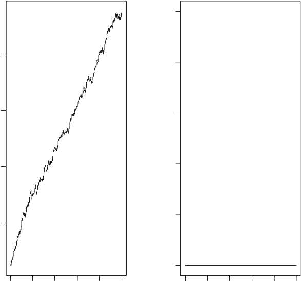
The output is shown in Figure 1.6. The effect of migration is so great that

the plot of population size is best shown on a log scale. Whereas the population

crashed quickly in the absence of migration, the presence of migration

prevents extinction and the population size increases to the unreasonably large

value of 10

Step 18: Controlling population growth: model 5

The mean population size reached after the addition of migration is unrealistic

but demonstrates the potential evolutionary importance of migration. Before

considering a model that allows migration rate to evolve we ﬁrst add a carrying

capacity to constrain population size.

1.4.6 Mathematical assumptions of model 5

1. All assumptions of model 4 apply to model 5 except that there is now a

limitation to population size.

2. Population size is limited to a maximum of 1,000 individuals.

Generation

02468

200 400 600 800 0 200 400 600 800

Mean population size

Number of pops extinct

Generation

Figure 1.6 Population size and number of extinct populations for model 4.

OVERVIEW 45

Assumption 2 is coded as

Npop[Npop>1000] <- 1000 # R code setting limit at 1000

Npop(Npop>1000) ¼ 1000; % MATLAB code setting limit at 1000

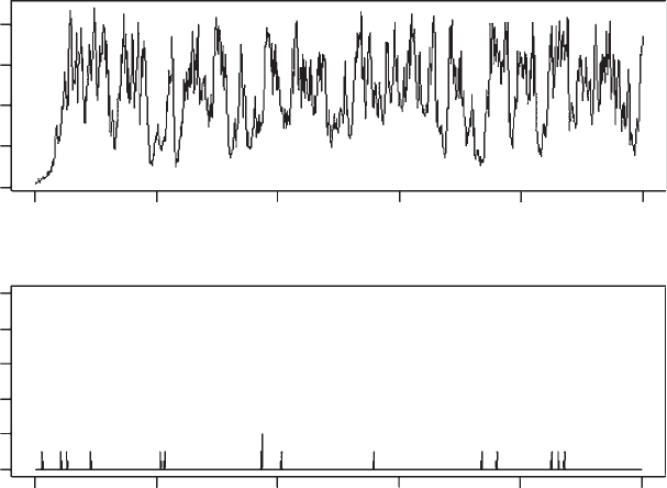
Incorporation of this restriction produces a dramatic drop in population size, an

increase in the number of temporally extinct populations, but no indication of a

signiﬁcant decline in population persistence (Figure 1.7). The mean population

size over the last 100 generations, obtained from the code mean (Npop.Sizes

[900:1000]) is only 473.2975, which is less than one half of the carrying capaci-

ty. Thus, the imposition of a carrying capacity in a heterogeneous environment

can have profound effects on population size even though a naive census would

suggest that the carrying capacity was not being exceeded (see Roff [1974a,

1974b]).

Step 19: More on graphics: functions expand.grid, outer, contour, persp

Many analyses will require investigation of effects due to variation in multiple

parameters: one method of graphically viewing such variation is to use a contour

plot and a 3-D perspective plot. There are several ways to generate such plot: here

I shall present two approaches. Before applying either method to the present

Generation

Number of pops extinct

Mean of population size

Generation

0 200 600

246810

200 400 600 800 1,000

0 200 400 600 800 1,000

Figure 1.7 Population size and number of extinct populations for model 5 (model 4 plus a

carrying capacity). For display purposes the graph page has been split horizontally using

par(mfcol=c(2,1)). Note that population size is not log transformed.

46 MODELING EVOLUTION

model I shall consider a much simpler model to better illustrate the procedures.

The object is to plot the equation of a circle:

z ¼

ﬃﬃﬃﬃﬃﬃﬃﬃﬃﬃﬃﬃﬃﬃﬃﬃ

þ y

;

 10 <x<10; 0 <y<10 ð1:35Þ

First we deﬁne the function for z.

R CODE:

FUNC.Z <- function(x,y) {sqrt(x^2þy^2)}

MATLAB CODE:

function z ¼ FUNC_Z(x,y)

z ¼ sqrt(x^2þy^2)

The ranges of x and y are divided into 10 parts (this will generate a matrix of 100

values):

R CODE:

n1 <-4;n2<-3

x <- seq(from¼10, to¼ 10, length¼n1)

y <- seq(from¼0, to ¼ 10, length¼n2)

MATLAB CODE:

n1 ¼ 4;

n2 ¼ 3;

x ¼ linspace(10, 10, n1);

y ¼ linspace(0, 10, n2);

Now we generate the matrix of z values for all combinations of x and y. In R this

can be done by either of the following:

1. Using the R function expand.grid which takes the two vectors and generates

a two-column matrix of all combinations, with the x variable changing most

rapidly:

d <-

expand.grid(x,y) # x values vary first

z <- FUNC.Z(d[,1], d[,2]) # Create z

The two-column matrix is now converted into the appropriate matrix:

z.matrix <- matrix(z,n1,n2)

2. An alternate method is to use the function outer

z.matrix <- outer(x, y, func.z)

The equivalent in MATLAB is meshgrid and rather than the function FUNC_Z

described above, I use here vectorization to give

OVERVIEW 47