Power electronic handbook

Подождите немного. Документ загружается.

1038 H. A. Toliyat et al.

voltage equation of the BLDC motor can be written as













R +pL

0 R +pL

00R +pL





















(37.2)

where v

, v

are the phase voltages, i

, i

are the phase

currents, e

, e

are the phase back-EMF voltages, R is the

phase resistance, L

is the synchronous inductance per phase

and includes both leakage and armature reaction inductances,

and p represents d/dt . The electromagnetic torque is given by

(

)

(37.3)

where ω

is the mechanical speed of the rotor. The equation

of motion is

(

−T

−Bω

)

(37.4)

where T

is the load torque, B is the damping constant, and J

is the moment of inertia of the rotor shaft and the load.

30 600 120 15090 210 240180 300 330270 360

Torque

Switches (T1-T6) turn on

Rotor position (Deg.)

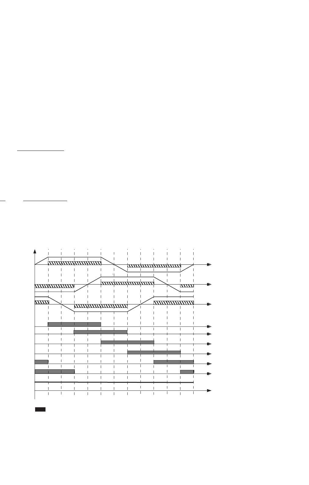
FIGURE 37.9 The principle of the six-step current control algorithm. T

–T

are the gate signals, E

, E

, and E

are the motor phase back-EMF, I

, and I

are the motor phase currents.

37.4.2 Torque Generation

From Eq. (37.3), the electromagnetic torque of the BLDC

motor is related to the product of the phase back-EMF and

current. The back-EMFs in each phase are trapezoidal in shape

and are displaced by 120 electrical degrees with respect to each

other in a three-phase machine. A rectangular current pulse

is injected into each phase so that current coincides with the

crest of the back-EMF waveform; hence the motor develops

an almost constant torque. This strategy, commonly called six-

step current control is shown Fig. 37.9. The amplitude of each

phase’s back-EMF is proportional to the rotor speed, and is

given by

E = kφω

(37.5)

where k is a constant and depends on the number of turns

in each phase, φ is the permanent magnet ﬂux, and ω

the mechanical speed. In Fig. 37.9, during any 120

◦

interval,

the instantaneous power converted from electrical to mechan-

ical, P

, is the sum of the contributions from two phases in

series, and is given by

= ω

= 2EI (37.6)

where T

is the output torque and I is the amplitude of the

phase current. From Eqs. (37.4) and (37.6), the expression for

37 DSP-based Control of Variable Speed Drives 1039

output torque can be written as

= 2kφI = k

I (37.7)

where K

is the torque constant. Since the electromagnetic

torque is only proportional to the amplitude of the phase

current in Eq. (37.7), torque control of the BLDC motor is

essentially accomplished by phase current control.

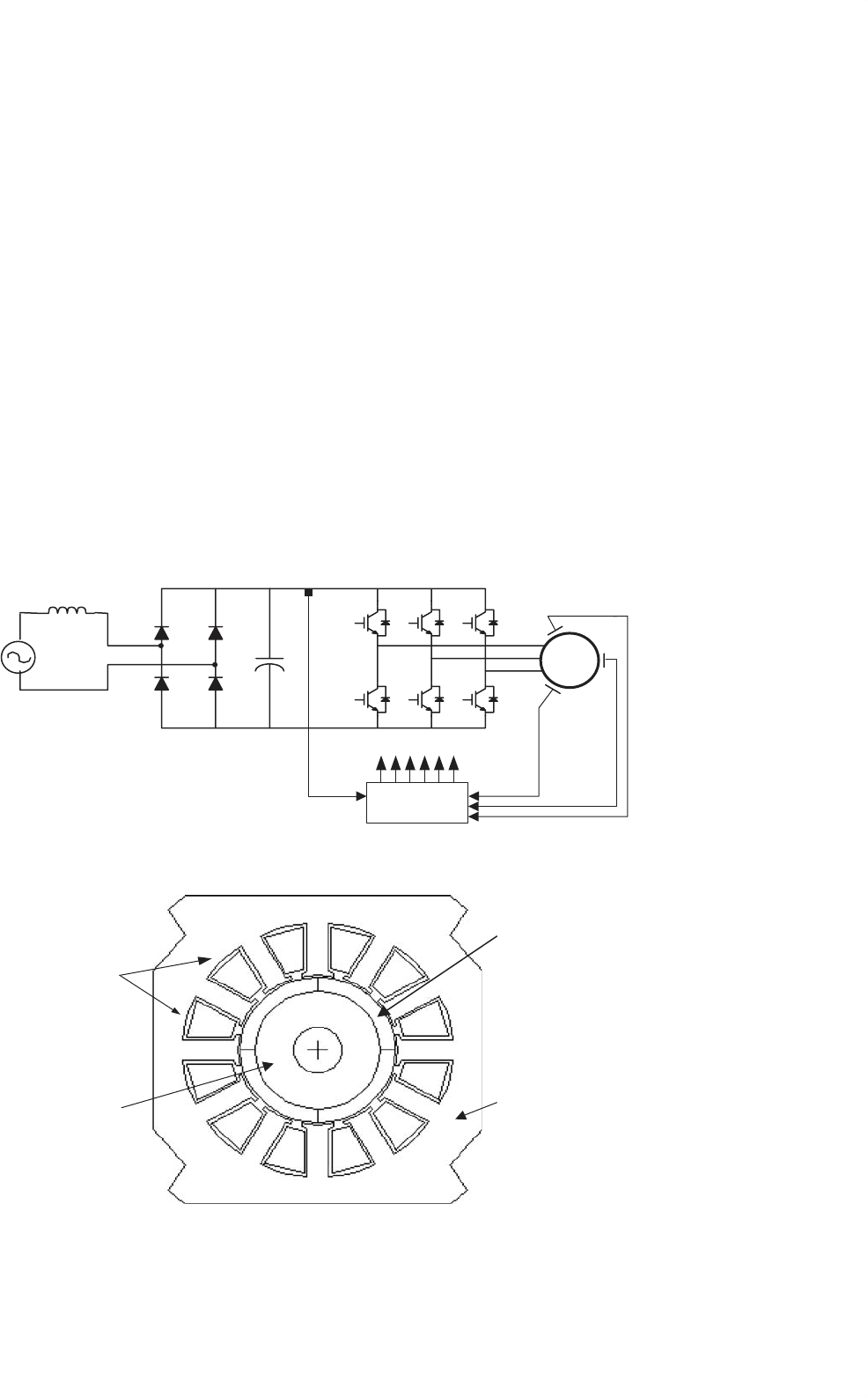
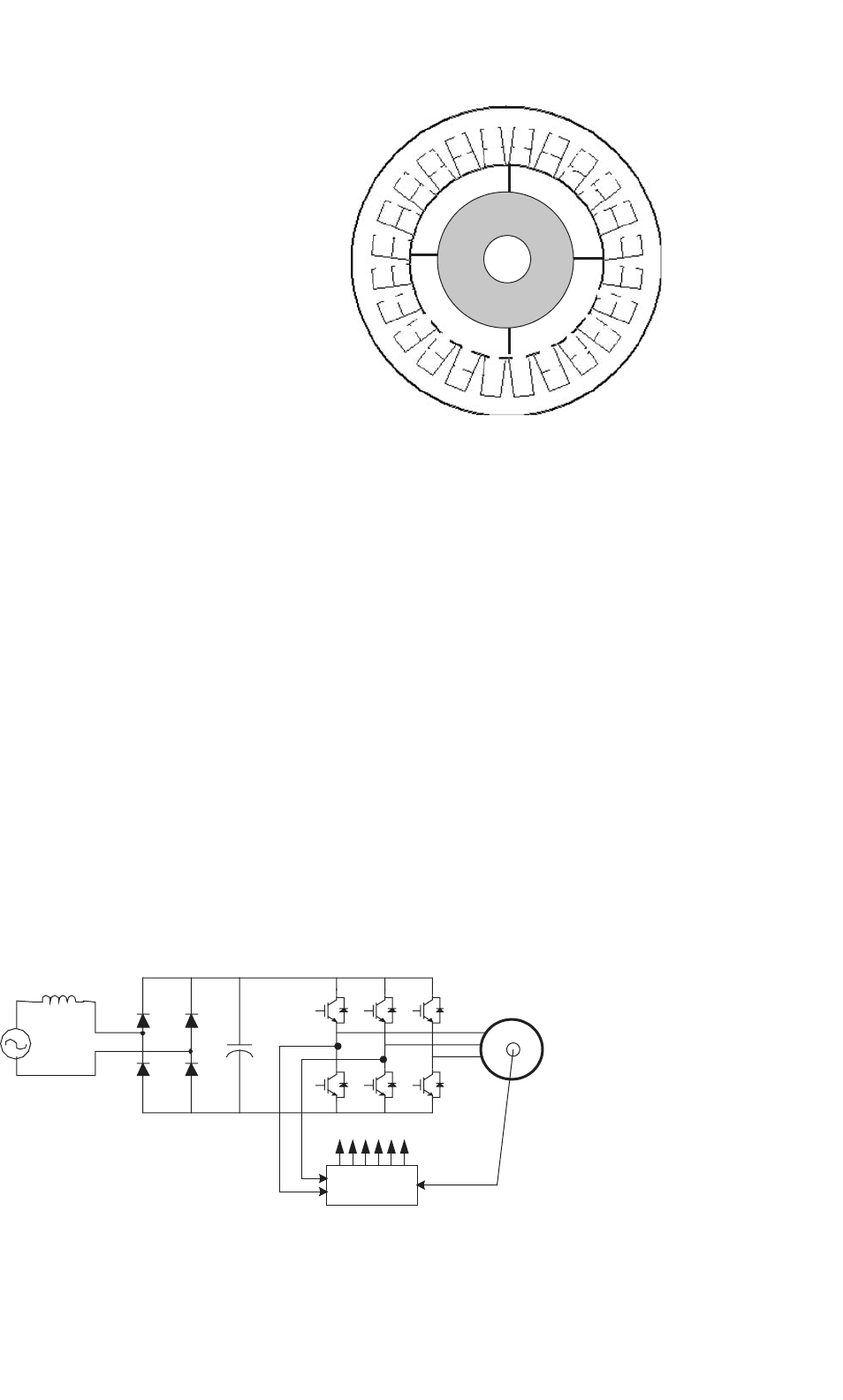
37.4.3 BLDC Motor Control Topology

Based on the previously discussed concept, a BLDC motor-

drive system is shown in Fig. 37.10. It can be seen that the total

drive system consists of the BLDC motor, power electronics

converter, sensor, and controller.

The BLDC motors are predominantly surface-magnet

machines with wide magnet pole arcs. The stator windings

are usually concentrated windings, which produce a square

waveform distribution of ﬂux density around the air-gap. The

design of the BLDC motor is based on the crest of each half-

cycle of the back-EMF waveform. In order to obtain a smooth

BLDC

Hall sensors

controller

DC-Bus

current

Gates T1 to T6

FIGURE 37.10 BLDC motor control system.

Permanent

Magnet

Stator

Windings

Rotor

A+

B+

C+

C−

A−

B−

FIGURE 37.11 The 4-pole 12-slot BLDC motor.

output torque, the back-EMF waveform should be wider than

120

◦

electrical degrees. A typical BLDC motor with 12 stator

slots and 4 poles on the rotor is shown in Fig. 37.11. The

inverter is usually responsible for the electronic commutation

and current regulation. For the six-step current control, if the

motor windings are Y-connected without the neutral connec-

tion, only two of the three phase currents ﬂow through the

inverter in series. This results in the amplitude of the DC link

current always being equal to that of the phase currents. The

PWM current controllers are typically used to regulate the

actual machine currents in order to match the rectangular

current reference waveforms shown in Fig. 37.9. For example,

during one 60

◦

interval, when switches T

and T

are active,

phases A and B conduct. The lower switch T

is always turned

on and the upper switch T

is chopped on/off using either a

hysteresis current controller with variable switch frequency or

a PI controller with ﬁxed switch frequency.

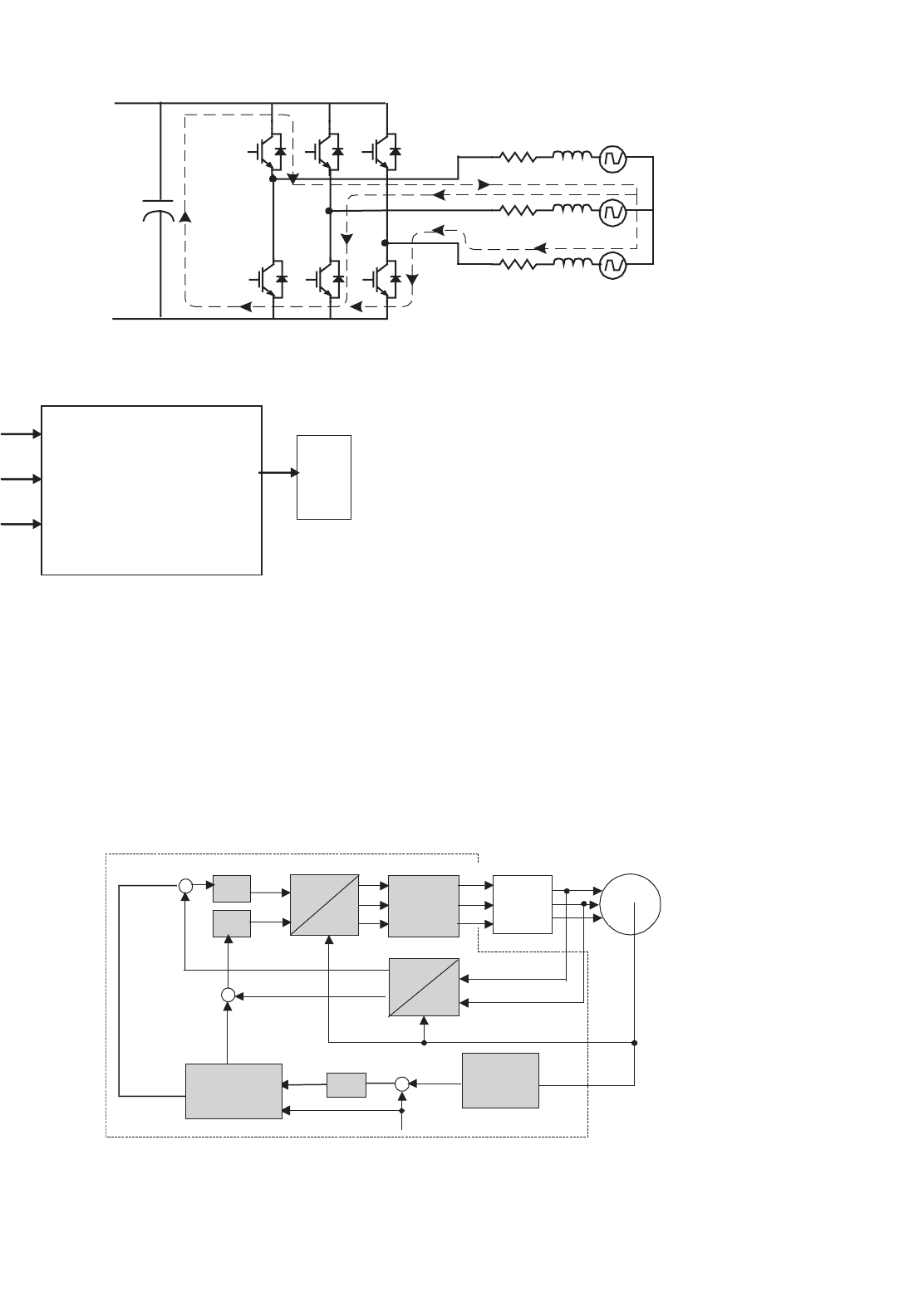
When T

and T

are conducting, current builds up in the

path as shown in Fig. 37.12a with dashed line. When switch T

is turned off, the current decays through diode D

and switch

as depicted in Fig. 37.12b. In the next interval, switch T

1040 H. A. Toliyat et al.

(a)

(b)

FIGURE 37.12 The current path when the switch T

turns on and turns off.

on, and T

is chopped so that phase A and phase C conduct.

During the commutation interval, the phase B current rapidly

decreases through the freewheeling diode D

until it becomes

zero and the phase C current builds up.

From the above analysis, each of the upper switches is

always chopped for one 120

◦

interval and the corresponding

lower switch is always turned on per interval. The freewheeling

diodes provide the necessary paths for the currents to circulate

when the switches are turned off and during the commuta-

tion intervals. There are two types of sensors for the BLDC

drive system: a current sensor and a position sensor. Since the

amplitude of the dc link current is always equal to the motor

phase current in six-step current control, the dc link current is

measured instead of the phase current. Thus, a shunt resistor,

which is in series with the inverter, is usually used as the cur-

rent sensor. Hall-effect position sensors typically provide the

position information needed to synchronize the stator excita-

tion with rotor position in order to produce constant torque.

Hall-effect sensors detect the change in magnetic ﬁeld. The

rotor magnets are used as triggers for the Hall sensors. A sig-

nal conditioning circuit is needed for noise cancellation in

Hall-effect sensors circuits. In six-step current control algo-

rithm, rotor position needs to be detected at only six discrete

points in each electrical cycle. The controller tracks these six

points so that the proper switches are turned on or off for the

correct intervals. Three Hall-effect sensors, spaced 120 elec-

trical degrees apart, are mounted on the stator frame. The

digital signals from the Hall sensors are then used to determine

the rotor position and switch gating signals for the inverter

switches.

37.4.4 DSP Controller Requirements

The controller of BLDC drive systems reads the current and

position feedback, implements the speed or torque control

algorithm, and ﬁnally generates the gate signals. The con-

nectivity of the LF2407 in this application is illustrated in

Fig. 37.13. Three capture units in the LF2407 are used to detect

both the rising and falling edges of Hall-effect signals. Hence,

every 60 electrical degrees of motor rotation, one capture unit

interrupt is generated which ultimately causes a change in the

gating signals and the motor to move to the next position. One

input channel of the 10-bit A/D converter reads the dc link

current. The output pins PWM1–PWM6 are used to supply

the gating signals to the inverter.

37 DSP-based Control of Variable Speed Drives 1041

TMS320F2407

PWM-1 &

PWM-6

ADCIN0I

Capture-1

Capture-2

Capture-2H2

Gate

Drive

FIGURE 37.13 The interface of LF2407.

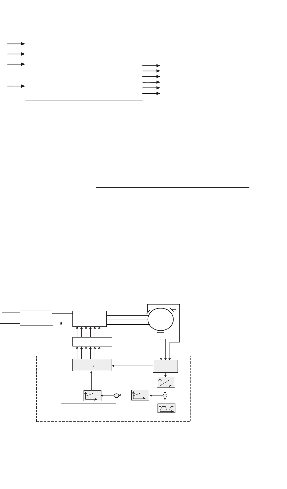
37.4.5 Implementation of the BLDC Motor

Control Algorithm Using LF2407

A block diagram of the BLDC motor control system is shown

in Fig. 37.14. The dashed line separates the software from the

hardware components introduced in the previous section. It is

necessary to choose hardware components carefully in order

to ensure high processing speed and precision in the overall

control system. The overall control algorithm of the BLDC

motor consists of nine modules:

• Initialization procedure

• Detection of Hall-effect signals

• Speed control subroutine

• Measurement of current

• Speed proﬁling

•

Calculation of actual speed

• PID regulation

• PWM generation

•

DAC output

BLDC

Firing

Circuit

Rectifier

Voltage

Source

~120 V

Integrator

Current PI

Controller

Speed PI

Controller

PWM

Generator

Hall

Signal

Hall_drv

Hall_state

ωf

−

LF2407

−

Speed Profile

FIGURE 37.14 The block diagram of BLDC motor control algorithm.

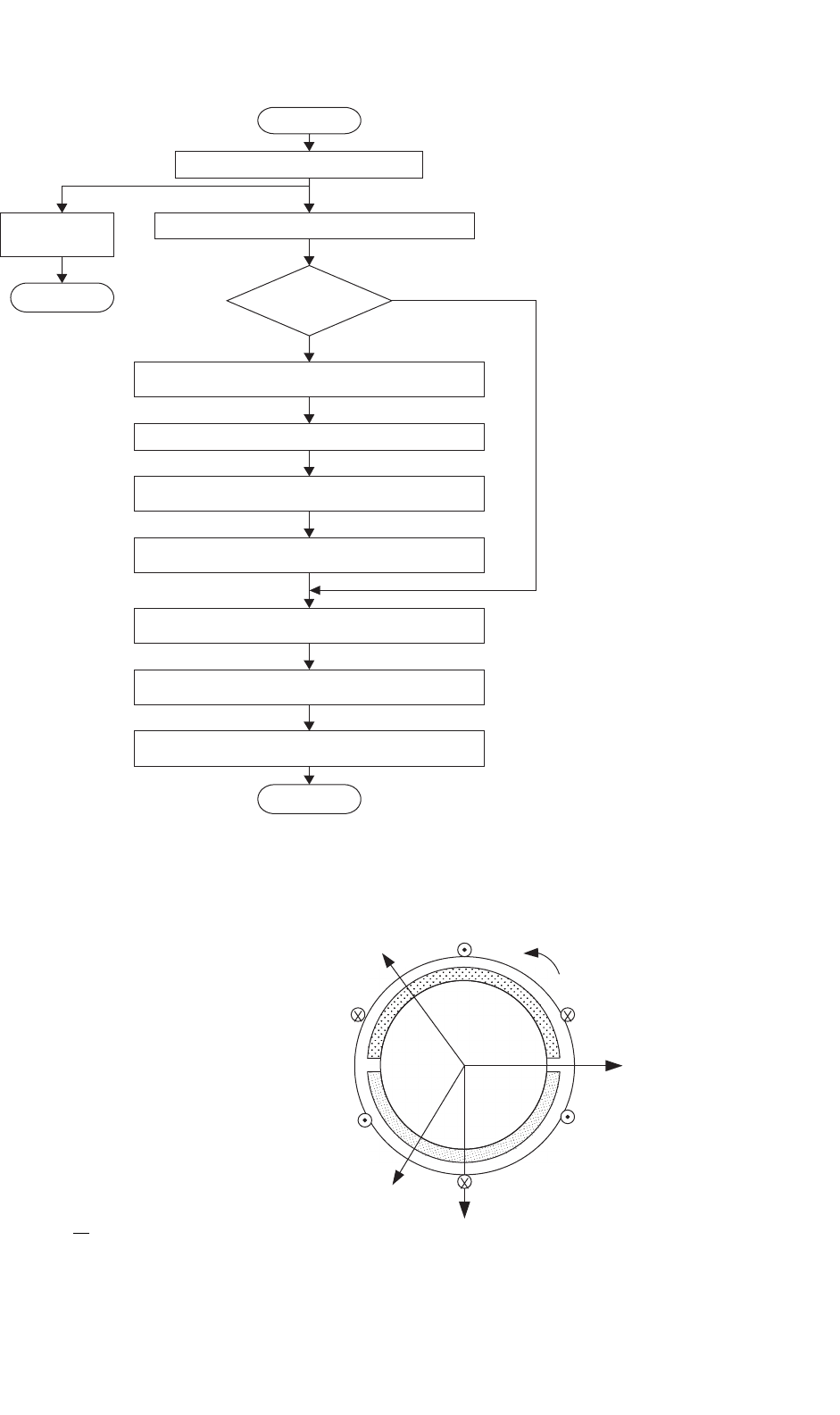
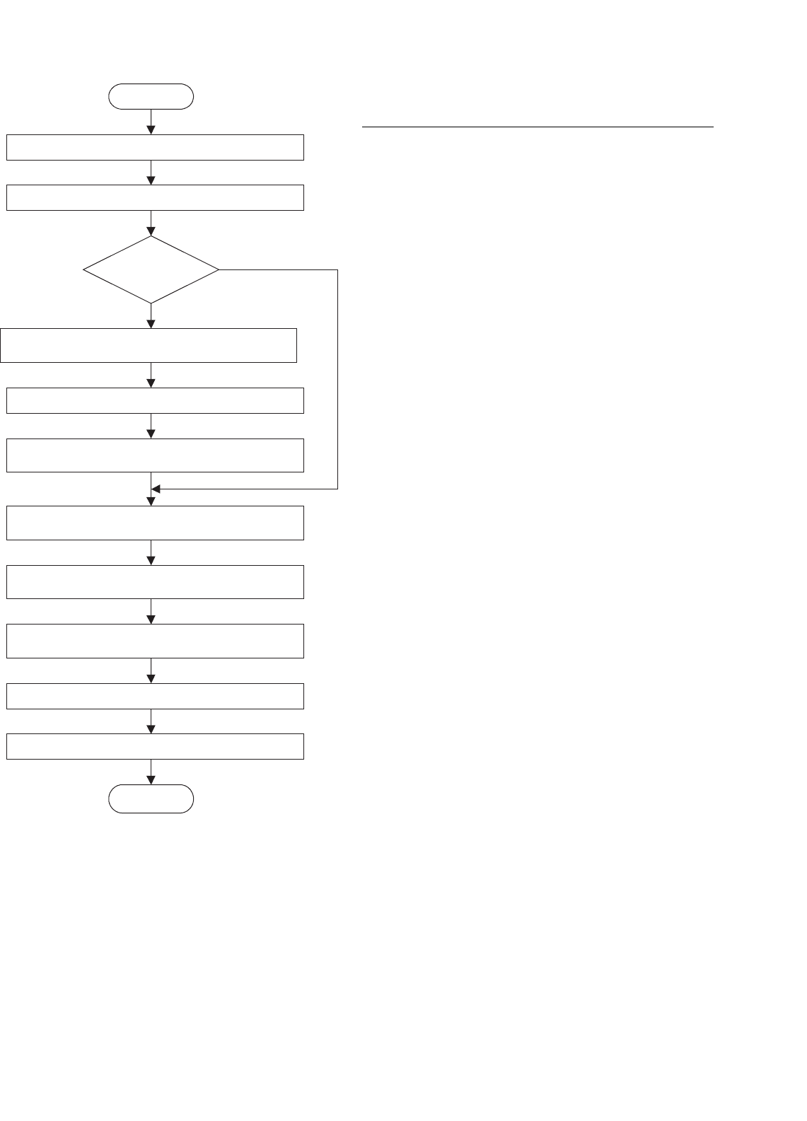
The ﬂowchart of the overall control algorithm is illustrated

in Fig. 37.15.

37.5 DSP-based Control of Permanent

Magnet Synchronous Machines

As previously described, the permanent magnet synchronous

motor (PMSM) is a PM motor with a sinusoidal back-EMF.

Compared to the BLDC motor, it has less torque ripple because

the torque pulsations associated with current commutation do

not exist. A carefully designed machine in combination with

a good control technique can yield a very low level of torque

ripple (<2% rated), which is attractive for high-performance

motor control applications such as machine tool and servo

applications.

In this section, following the same procedures used in the

previous section, the principles of the PMSM drive system will

1042 H. A. Toliyat et al.

Read DC link current I

; Load Hall Effect signals

Start

Initialization procedure

Execute

speed loop?

Read reference speed w

ref

Read Hall

sensor signal

End

Yes

Calculate the motor actual speed w

Speed PI regulator

Calculate the commended torque

Current PI regulator

Generate the PWM using ∆ generator

End

Output the program variables to DAC0~DAC3

Calculate the command DC link current i

using (28.7)

FIGURE 37.15 BLDC algorithm ﬂowchart.

be introduced. Later, the control implementation using the

LF2407 DSP will be described in detail.

37.5.1 Mathematical Model of PMSM

Figure 37.16 depicts the simpliﬁed three-phase surface

mounted PMSM motor for our discussion. The stator wind-

ings, as–as



, bs–bs



, and cs–cs



, are shown as lumped windings

for simplicity, but are actually distributed around the stator.

The rotor has 2 poles. Mechanical rotor speed and position are

denoted as ω

and θ

, respectively. Electrical rotor speed and

position, ω

and θ

, are deﬁned as P/2 times the corresponding

mechanical quantities, where P is the number of poles.

Based on the above motor deﬁnition, the voltage equation

in the abc stationary reference frame is given by

abcs

= R

abcs

(37.8)

as'

bs'

cs'

A-axis

B-axis

C-axis

Wrm

d-axis

q-axis

FIGURE 37.16 The cross section of PMSM.

37 DSP-based Control of Variable Speed Drives 1043

where

abcs





(37.9)

and the stator resistance matrix is given by

= diag[

]

(37.10)

The ﬂux linkages equation can be expressed by

abcs

= L

abcs

+λ









sin ϑ

sin(ϑ

−

2π

)

sin(ϑ

−

4π

)







(37.11)

where λ



denotes the amplitude of the ﬂux linkages estab-

lished by the permanent magnet as viewed from the stator

phase windings. Note that in Eq. (37.11) the back-EMFs are

sinusoidal waveforms that are 120

◦

apart from each other.

The stator self-inductance matrix, L

, is given as







−L

cos 2θ

−

−L

cos 2(θ

−π/3) −

−L

cos 2(θ

+π/3)

−

−L

cos 2(θ

−π/3) L

−L

cos 2(θ

−2π/3) −

−L

cos 2(θ

+π)

−

−L

cos 2(θ

+π/3) −

−L

cos 2(θ

+π) L

−L

cos 2(θ

+2π/3)







(37.12)

The torque and speed are related by the electromechanical

motion equation

−T

) −B

(37.15)

where J is the rotational inertia, B

is the approximated

mechanical damping due to friction, and T

is the load torque.

37.5.2 Mathematical Model of PMSM in Rotor

Reference Frame

The voltage and torque equations can be expressed in the rotor

reference frame in order to transform the time-varying vari-

ables into steady-state constants. The transformation of the

three-phase variables in the stationary reference frame to the

rotor reference frame is deﬁned as

qd0r

= K

abcs

(37.16)

where







cos θ

cos(θ

−

2π

) cos(θ

2π

)

sin θ

sin(θ

−

2π

) sin(θ

2π

)







If the applied stator voltages are given by











√

cos θ

√

cos(θ

−

2π

)

√

cos(θ

2π

)

(37.17)

Then applying (37.16) to (37.8), (37.11), and (37.17) yields

= r

+ω

(37.18)

= r

−ω

(37.19)

= L

(37.20)

= L

+λ



(37.21)

where the q- and d-axes self-inductances are given by

= L

and L

= L

, respectively.

The electromagnetic torque can be written as

[λ



+(L

−L

] (37.22)

The electromagnetic torque may be written as







−

)cosθ

−

√

−i

)sinϑ



−L



−

−i

+2i

)

sin2θ

√



−2i

+2i



cos2θ



cog

(θ

)

(37.13)

In Eq. (37.13), T

cog

(θ

) represents the cogging torque and

the d- and q-axes magnetizing inductances are deﬁned by

−L

)

and

) (37.14)

1044 H. A. Toliyat et al.

From Eq. (37.22), it can be seen that torque is related only

to the d- and q-axes currents. Since L

≥ L

(for surface

mount PMSM both inductances are equal), the second item

contributes a negative torque if the ﬂux weakening control has

been used. In order to achieve the maximum torque/current

ratio, the d-axis current is set to zero during the constant

torque control so that the torque is proportional only to the

q-axis current. Hence, this results in the control of the q-axis

current for regulating the torque in rotor reference frame.

37.5.3 PMSM Control Topology

Based on the above analysis, a PMSM drive system is developed

as shown in Fig. 37.17. The total drive system looks similar to

that of the BLDC motor and consists of a PMSM, power elec-

tronics converter, sensors, and controller. These components

are discussed in detail in the following sections.

The design consideration of the PMSM is to ﬁrst generate

the sinusoidal back-EMF. Unlike the BLDC, which needs con-

centrated windings to produce the trapezoidal back-EMF, the

stator windings of PMSM are distributed in as many slots per

pole as deemed practical to approximate a sinusoidal distri-

bution. To reduce the torque ripple, standard techniques such

as skewing and chorded windings are applied to the PMSM.

With the sinusoidally excited stator, the rotor design of the

PMSM becomes more ﬂexible than the BLDC motor where the

surface-mount permanent magnet is a favorite choice. Besides

the common surface-mount non-salient pole PM rotor, the

salient pole rotor, like inset and buried magnet rotors, are

often used because they offer appealing performance charac-

teristics during the ﬂux weakening region. A typical PMSM

with 36 stator slots in stator and 4 poles on the rotor is shown

in Fig. 37.18.

Due to the sinusoidal nature of the PMSM, control algo-

rithms such as V/f and vector control, developed for other AC

motors, can be directly applied to the PMSM control system. If

the motor windings are Y-connected without a neutral connec-

tion, three-phase currents can ﬂow through the inverter at any

Controller

to T1~T6

PMSM

ias

ibs

Resolver

FIGURE 37.17 The PMSM speed control system.

−C

−A

−B

−C

−B

FIGURE 37.18 A 4-pole 24-slot PMSM.

moment. With respect to the inverter switches, three switches,

one upper and two lower in three different legs conduct at any

moment as shown in Fig. 37.19. The PWM current control is

still used to regulate the actual machine current. Either a hys-

teresis current controller, a PI controller with sine-triangle, or

an SVPWM strategy is employed for this purpose. Unlike the

BLDC motor, the three switches are switched at any time.

37.5.4 DSP Controller Requirements

The LF2407 is used as the controller to implement speed con-

trol of the PMSM system. The interface of the LF2407 is

illustrated in Fig. 37.20. Similar to the BLDC motor control

system, three input channels are selected to read the two-

phase currents and resolver signal. Because a resolver is used

in one case, the quadrature-encoder-pulse (QEP) inputs are

not used. The QEP inputs work only with a QEP signal that a

rotary encoder supplies. The DSP output pins PWM1–PWM6

used to supply the gating signals to the switches and form the

output of the control part of the system.

37 DSP-based Control of Variable Speed Drives 1045

FIGURE 37.19 The current path when the three phases are chopped.

Gate

Drive

PWM-1 to

PWM-6

TMS320LF2407

ADCIN0

ADCIN1

ADCIN2

FIGURE 37.20 The interface of LF2407.

37.5.5 Implementation of the PMSM Algorithm

Using the LF2407

The block diagram of the PMSM drive system is displayed in

Fig. 37.21.

The ﬂowchart of the developed software is shown in

Fig. 37.22. The control program of the PMSM has one main

Software

ref

−

Vbs

Vcs

Vas

qsr

dsr

qsr

dsr

ibs

ias

PWM

Inverter

d, q

a, b ,c

PWM

Generator

d, q

a b,c

= 0

dsr

qsr

−

Speed

calculator

Current

calculator

FIGURE 37.21 Block diagram of PMSM speed control system.

routine and includes four modules:

•

Initialization procedure

• DAC module

• ADC module

• Speed control module

In the following section speed control module is disscussed.

37.5.5.1 The Speed Control Algorithm

The requirement for speed control algorithm can be item-

ized as:

• Reading the current and position signal, then generating

the commanded speed proﬁle

• Calculating the actual motor speed, transferring the

variables in the abc model to the d–q model and reverse

• Regulating the motor speed and currents using the

vector-control strategy

1046 H. A. Toliyat et al.

Yes

Start

Initialization procedure

Read phase current i

; read the position signal;

Execute

speed loop?

Set reference speed w

ref

and calculate the actual speed

Speed PI regulator used to calculate the commend torque

Calculate the command q-axis current i

; Set i

Current PI regulator used to calculate the v

in RRF

Transfer i

to i

in Rotor Reference Frame (RRF)

Transfer v

in RRF to v

Generate the PWM using sine-

generator

End

Output the program variables to DAC0~DAC3

FIGURE 37.22 The ﬂowchart of PMSM control system.

•

Generating the PWM signal based on the calculated

motor phase voltages

The PWM frequency is determined by the time interval

of the interrupt, with the controlled phase voltages being

recalculated every interrupt.

37.6 DSP-based Vector Control of

Induction Motors

For many years, induction motors have been preferred for

a variety of industrial applications because of their robust

and rugged construction. Compared to dc motors, induction

motors are not as easy to control. They typically draw large

starting currents, about six to eight times their full load values,

and operate with lagging power factor when loaded. However,

with the advent of the vector-control concept for motor con-

trol, it is possible to decouple the torque and the ﬂux, thus

making the control of the induction motor very similar to that

of the dc motor.

The most popular type of induction motor used is the squir-

rel cage induction motor. The rotor consists of a laminated

core with parallel slots for carrying the rotor conductors, which

are usually heavy bars of copper, aluminum, or alloys. One bar

is placed in each slot; or rather, the bars are inserted from the

end when the semi-closed slots are used. The rotor bars are

brazed, electrically welded, or bolted to two heavy and stout

short-circuiting end-rings, thus completing the squirrel cage

construction. The rotor bars are permanently short-circuited

on themselves. The rotor slots are usually not parallel to the

shaft, but are given a slight angle, called a skew, which increases

the rotor resistance due to increased length of rotor bars and an

increase in the slip for a given torque. The skew is also advan-

tageous because it reduces the magnetic hum while the motor

is operating and reduces the locking tendency, or cogging, of

the rotor teeth.

When the three-phase stator windings are fed by a three-

phase supply, a magnetic ﬂux of a constant magnitude rotating

at synchronous speed is created in the air-gap. Due to the

relative speed between the rotating ﬂux and the stationary

conductors, an electromagnetic force (EMF) is induced in the

rotor in accordance with Faraday’s laws of electromagnetic

induction. The frequency of the induced EMF is the same as

the supply frequency, and the magnitude is proportional to the

relative velocity between the ﬂux and the conductors. There-

fore, the rotor current develops in the same direction as the

ﬂux and tries to catch up with the rotating ﬂux.

37.6.1 Induction Motor Field-oriented Control

The term “vector” control refers to the control technique that

controls both the amplitude and the phase of ac excitation

voltage. Vector control controls the spatial orientation of the

EMF in the machine. This has led to the coining of the term

FOC, which is used for controllers that maintain a 90

◦

spatial

orientation between the critical ﬁeld components.

The required 90

◦

of spatial orientation between key ﬁeld

components can be compared to the dc motor, where the

armature winding magnetic ﬁeld and the ﬁled winding mag-

netic ﬁled are always in quadrature. The objective is to force

37 DSP-based Control of Variable Speed Drives 1047

the control of the induction machine to be similar to the con-

trol of a dc motor, i.e., torque control. In dc machines, the

ﬁeld and the armature winding axes are orthogonal to one

another, making the magnetomotive forces (MMFs) estab-

lished orthogonal. If the iron saturation is ignored, then

the orthogonal ﬁelds can be considered to be completely

decoupled.

It is important to maintain a constant ﬁeld ﬂux for proper

torque control. It is also important to maintain an indepen-

dently controlled armature current in order to overcome the

effects of the detuning of resistance of the armature winding,

and leakage inductance. A spatial angle of 90

◦

between the ﬂux

and MMF axes has to be maintained in order to limit inter-

action between the MMF and the ﬂux. If these conditions are

met at every instant of time, the torque will always follow the

current.

With vector control, the mechanically robust induction

motors can be used in high-performance applications where

dc motors were previously used. The key feature of the control

scheme is the orientation of the synchronously rotating q–d–0

frame to the rotor ﬂux vector. The d-axis component is aligned

with the rotor ﬂux vector and regarded as the ﬂux-producing

current component. On the other hand, the q-axis current,

which is perpendicular to the d-axis, is solely responsible for

torque production.

In order to apply a rotor ﬂux ﬁeld-orientation condition,

the rotor ﬂux linkage is aligned with the d-axis, so the q-axis

rotor ﬂux in excitation reference frame λ

will be zero and

the d-axis rotor ﬂux in the excitation reference frame will be

the rotor ﬂux; λ

. Therefore we have:

(37.23)

slip





(37.24)

(37.25)

where τ

is rotor time constant, L

is magnetizing inductance,

rotor leakage inductance, r

rotor resistance, i

q-axis stator

current in excitation frame, i

d-axis stator current in exci-

tation frame, and ω

slip

angular frequency of slip. We can ﬁnd

out that in this case i

controls the rotor ﬂux linkage and i

controls the electromagnetic torque. The reference currents of

the q–d–0 axis (i

e∗

, i

e∗

) are converted to the reference phase

voltages (v

e∗

, v

e∗

) as the commanded voltages for the con-

trol loop. Given the position of the rotor ﬂux and two-phase

currents, this generic algorithm implements the instantaneous

direct torque and ﬂux control by means of coordinate trans-

formations and PI regulators, thereby achieving accurate and

efﬁcient motor control.

It is clear that for implementing vector control we have to

determine the rotor ﬂux position. This usually is performed by

measuring the rotor position and utilizing the slip relation to

compute the angle of the rotor ﬂux relative to the rotor axis.

Equations (37.23) and (37.24) show that we can control

torque and ﬁeld by i

and i

in the excitation frame. However,

in the implementation of FOC, we need to know i

and i

in the stationary reference frame. So, we have to know the

angular position of the rotor ﬂux to transform i

and i

from

the excitation frame to the stationary frame. By using ω

slip

which is shown in Eq. (37.24) and using actual rotor speed,

the rotor ﬂux position is obtained.



slip

dt +θ

(t) = θ

(t) (37.26)

Where θ

(t) is electrical angular rotor position, and θ

(t)

angular rotor ﬂux position.

The Current Model takes i

and i

as inputs as well as the

rotor mechanical speed and gives the rotor ﬂux position as an

output. Figure 37.23 shows the block diagram of the vector-

control strategy in which speed regulation is possible using a

control loop.

As shown in Fig. 37.23, two-phase currents are measured

and fed to the Clarke transformation block. These projection

outputs are indicated as i

and i

. These two components

of the current provide the inputs to Park’s transformation,

which gives the currents in the qds

excitation reference frame.

The i

and i

components, which are outputs of the Park

transformation block, are compared to their reference val-

ues i

e∗

, the ﬂux reference, and i

e∗

, the torque reference. The

torque command, i

e∗

, comes from the output of the speed

controller. The ﬂux command, i

e∗

, is the output of the ﬂux

controller which indicates the right rotor ﬂux command for

every speed reference. For i

e∗

, we can use the fact that the

magnetizing current is usually between 40 and 60% of the

nominal current. For operating in speeds above the nomi-

nal speed, a ﬁeld weakening section should be used in the

ﬂux controller section. The current regulator outputs, v

e∗

and v

e∗

, are applied to the inverse Park transformation. The

outputs of this projection are v

and v

, which are the com-

ponents of the stator voltage vector in the dqs

orthogonal

reference frame. They form the inputs of the space-vector

PWM block. The outputs of this block are the signals that

drive the inverter.

Note that both the Park and the inverse Park transforma-

tions require the exact rotor ﬂux position, which is given by

the Current Model block. This block needs the rotor resistance

or rotor time constant as a parameter. Accurate knowledge of

the rotor resistance is essential to achieve the highest possible

efﬁciency from the control structure. Lack of this knowledge

results in the detuning of the FOC. In Fig. 37.23, a space-

vector PWM has been used to emulate v

and v

in order to

implement current regulation.