Murota K. Matrices and Matroids for Systems Analysis

Подождите немного. Документ загружается.

402 6. Theory and Application of Mixed Polynomial Matrices





(γ =1)

(−1)

(0)

(−1)

(γ =1)

(γ =0)

(0)

(γ =0)



(γ =0)

(−1)

(1)

(γ =0)

(0)

(γ = −1)

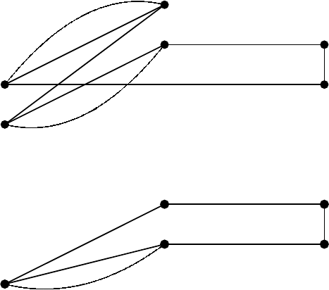
Fig. 6.11. Strong components free from E

in Example 6.5.17 (

admits a po-

tential and

does not)

D(s)=

⎡

⎣

−sb 0

0 −10

c 0 −1

⎤

⎦

⎡

⎣

−s 00

0 −10

00−1

⎤

⎦

⎡

⎣

0 b 0

000

c 00

⎤

⎦

⎡

⎣

000

⎤

⎦

to obtain the auxiliary network N =(G, γ)for(

J)=(∅, ∅). The graph G

is acyclic, and each strong component, consisting of a single vertex, admits

a potential function in a trivial manner. By Theorem 6.5.15 we can conclude

that there exists no nonzero ﬁxed mode. The existence of a zero ﬁxed mode is

exhibited by (I,J)=({x, u}, {x, y}) in Theorem 6.5.12(iii), where Row(D)=

Col(D)={x, u, y}. 2

Example 6.5.19. The present method successfully detects the zero ﬁxed

mode in Example 6.5.9, which is overlooked by the graph-theoretic method.

We take the matrix of (6.96) with n =6,m =3,andl = 6 as the matrix

(s) of size 15, which turns out to satisfy (MP-Q2) with

, ···,r

)=(1, 1, 1, 2, 1, 2; 0, 0, 0; 0, 0, 0, 1, 0, 1),

, ···,c

)=(0, 0, 0, 1, 0, 1; 0, 0, 0; 0, 0, 0, 1, 0, 1).

Then Theorem 6.5.12 reveals the existence of the zero ﬁxed mode. 2

Notes. The mixed matrix formulation in §6.5.3 and the algorithm in §6.5.4

are taken from Murota [209].

7. Further Topics

This chapter introduces three supplementary, mutually independent, topics:

the combinatorial relaxation algorithm, combinatorial system theory, and

mixed skew-symmetric matrices.

7.1 Combinatorial Relaxation Algorithm

The “combinatorial relaxation” approach to algebraic computation initiated

by Murota [212] is described here for the problem of computing the maxi-

mum degree of subdeterminants of a polynomial/rational matrix, the prob-

lem treated in §6.2 by graph-theoretic and valuated matroid-theoretic meth-

ods. A purely combinatorial algorithm, whether graph-theoretic or matroid-

theoretic, is based on a genericity assumption, and hence can possibly fail

when the assumed genericity is not satisﬁed by speciﬁc input data. An al-

gorithm of “combinatorial relaxation” type is a remedy for this. It always

returns the correct answer, while sharing the spirit of generic approach. It

is eﬃcient, behaving as a combinatorial algorithm in most cases, and at the

same time it is reliable, coping with nongeneric cases where numerical can-

cellation does aﬀect the answer.

7.1.1 Outline of the Algorithm

Let A(s)=(A

(s)) be an m × n rational function matrix with A

(s) being

a rational function in s with coeﬃcients from a certain ﬁeld F (typically

the real number ﬁeld R). We shall present an algorithm for computing the

highest degree of a minor of order k of A(s):

(A) = max{deg

det A[I,J] ||I| = |J| = k}. (7.1)

As a combinatorial counterpart of δ

(A) we consider the maximum weight of

a k-matching in the associated bipartite graph G(A)=(V,E) introduced in

§6.2.2; each arc of G(A) corresponds to a nonzero entry A

(s) and is given

a weight w

= deg

(s). We then deﬁne

(A) = max{w(M) | M is a k-matching in G(A)}, (7.2)

K. Murota, Matrices and Matroids for Systems Analysis,

Algorithms and Combinatorics 20, DOI 10.1007/978-3-642-03994-2

 Springer-Verlag Berlin Heidelberg 2010

404 7. Further Topics

where

(A)=−∞ if no k-matching exists.

As has been discussed in §6.2.2 (Theorem 6.2.2 in the case of a polyno-

mial matrix), the combinatorial value

(A) is an upper bound on δ

(A)and

it is generically tight. Recall that the word “generic” refers to an algebraic

assumption that the nonzero coeﬃcients in A(s) are subject to no algebraic

relations, whereas its practical interpretation would be “so long as no acci-

dental numerical cancellation occurs.” To make this statement more precise,

we deﬁne an m × n constant matrix A

◦

=(A

◦

)by

◦



lim

s→∞

−w

(s)ifA

(s) =0

0ifA

(s)=0.

(7.3)

Let us call A

◦

the leading coeﬃcient of A

(s), since, when A

(s) is a poly-

nomial, A

◦

is equal to the coeﬃcient of the highest-degree term in A

(s).

Theorem 7.1.1. Let A(s) be a rational function matrix.

(1) δ

(A) ≤

(A).

(2) The equality holds generically, i.e., if the set of nonzero leading coef-

ﬁcients {A

◦

| A

◦

=0} is algebraically independent (over a subﬁeld of F ).

We say that A(s)isupper-tight (for k)ifδ

(A)=

(A). Note that genericity

is suﬃcient and not necessary for the upper-tightness.

The algorithm, outlined below, takes advantage of two facts:

(i)

(A) is generically equal to δ

(A), and

(ii)

(A) can be computed eﬃciently by a combinatorial algorithm.

The algorithm ﬁrst computes

(A), instead of δ

(A), by solving a weighted-

matching problem using an eﬃcient combinatorial algorithm (Phase 1), and

then checks whether

(A) equals δ

(A) (Phase 2). The algorithm invokes an

exception-handling algebraic elimination routine to modify A only when it

detects discrepancy between

(A)andδ

(A) due to numerical cancellation

(Phase 3). In Phase 3, where δ

(A) ≤

(A) −1, the matrix A is modiﬁed to

another matrix A



such that δ



)=δ

(A)and



) ≤

(A) − 1.

Algorithm for computing δ

(A) (outline)

Phase 1 : Compute

(A) by solving the weighted-matching problem in G(A)

using an eﬃcient combinatorial algorithm (cf. Ahuja–Magnanti–Orlin [3],

Cook–Cunningham–Pulleyblank–Schrijver [40], Lawler [171]).

Phase 2 : Test whether δ

(A)=

(A) or not (without computing δ

(A)).

If so, output

(A) and stop.

Phase 3 : Modify A to another matrix A



such that δ



)=δ

(A)and



) ≤

(A) − 1. Put A := A



andgotoPhase1. 2

7.1 Combinatorial Relaxation Algorithm 405

The test in Phase 2 for the upper-tightness can be reduced to computing

the ranks of four constant matrices (see Theorem 7.1.9). The modiﬁcation

algorithm of Phase 3, to be described in detail in §7.1.3, makes essential use of

dual variables based on the duality theorem for the polyhedral description of

matchings. Since numerical cancellation occurs only rarely (or nongenerically)

the above algorithm is combinatorial in almost all cases and hence suitable

for large scale problems.

Remark 7.1.2. In more general terms an algorithm of “combinatorial re-

laxation” type consists of the following three distinct phases:

Phase 1: Consider a relaxation (or an easier problem) of a combinatorial

nature to the original problem and ﬁnd a solution to the relaxed problem.

Phase 2: Test for the validity of this solution to the original problem (without

computing the solution to the original problem).

Phase 3 (In case of invalid solution): Modify the relaxation so that the

invalid solution is eliminated.

It is crucial for computational eﬃciency that the relaxed problem can be

solved eﬃciently and that the modiﬁcation of the relaxation in Phase 3 need

not be invoked many times. 2

Example 7.1.3. Some technical issues of the combinatorial relaxation algo-

rithm above are illustrated here for a speciﬁc example. Consider a polynomial

matrix over F = R (m = n = 4):

A(s)=

⎛

⎜

⎝

αs

02s

+1 s

+ ss

−s

s 0 s +2

⎞

⎟

⎠

with a nonzero parameter α introduced for an illustrative purpose. The as-

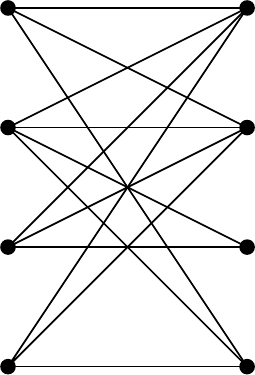
sociated bipartite graph G = G(A), shown in Fig. 7.1, has 8 vertices and 13

arcs. The leading coeﬃcient matrix (7.3) is given by

◦

⎛

⎜

⎝

α 102

1111

11−10

2101

⎞

⎟

⎠

. (7.4)

Let us consider the minors of order k = 3, and assume α = 1 as the

ﬁrst case. We may take, for example, M

(1)

= {(r

), (r

)} as

a matching of size 3 of maximum weight w(M

(1)

) = 3 + 6 + 4 = 13. The

corresponding submatrix

406 7. Further Topics

Fig. 7.1. Bipartite graph G(A) (Example 7.1.3)

A[∂

(1)

,∂

−

(1)

⎛

⎝

αs

+1 s

+ ss

⎞

⎠

has another matching M

(2)

= {(r

), (r

)} of weight w(M

(2)

3 + 5 + 5 = 13. In the determinant expansion of this minor, the two terms of

degree 13 arising from M

(1)

and M

(2)

cancel each other, and

det A[{r

}, {c

}]=(1− α)s

− 2s

+ s

− 2s

Therefore,

(A[{r

}, {c

}]) = 11

< 13 = w(M

(1)

(A[{r

}, {c

}]).

Nevertheless, we have δ

(A)=13=

(A), provided α = 1, because

of the existence of another minor of degree 13. Consider a third matching

(3)

= {(r

), (r

)} of weight w(M

(3)

) = 5 + 5 + 3 = 13. The

corresponding submatrix

A[∂

(3)

,∂

−

(3)

⎛

⎝

αs

+1 s

+ ss

−s

⎞

⎠

7.1 Combinatorial Relaxation Algorithm 407

admits four matchings (of size 3) of weight 13, and has the determinant

det A[{r

}, {c

}] = 2(1 − α)s

+ s

− αs

Hence δ

(A)=13=

(A), provided α =1.

The phenomenon observed above illustrates a challenging complication:

after we have found a matching M of maximum weight in Phase 1, we must

look globally for a k×k minor of degree w(M ) before we can decide in Phase 2

whether w(M) is equal to δ

(A) or not.

In case α = 1 we can verify by inspection that there exists no 3 × 3

minor of degree equal to 13, whereas deg

det A[{r

}, {c

}] = 12.

Accordingly we conclude

(A)=13,δ

(A)=



13 if α =1

12 if α =1.

The values of

(A)andδ

(A)fork =1, 2, 4 can be found similarly:

(A)=6,δ

(A)=6,

(A)=10,δ

(A)=



10 if α =1

9ifα =1,

(A)=14,δ

(A)=



14 if α =5

13 if α =5.

7.1.2 Test for Upper-tightness

This section describes a procedure for Phase 2 which tests for the upper-

tightness δ

(A)=

(A)ofA(s) without computing δ

(A). The procedure

makes use of the standard duality result for bipartite matchings, which follows

from the integrality of the associated linear programs.

We consider the following primal-dual pair of linear programs (Chv´atal

[35], Lawler [171], Lov´asz–Plummer [181], Schrijver [292]):

PLP(k): Maximize



e∈E

subject to



∂ei

≤ 1(i ∈ V ), (7.5)



e∈E

= k,

≥ 0(e ∈ E);

DLP(k): Minimize



i∈V

+ kq (≡ π(p, q)),

subject to p

+ p

+ q ≥ w

((i, j) ∈ E), (7.6)

≥ 0(i ∈ V ).

408 7. Further Topics

Note that ξ =(ξ

| e ∈ E) ∈ R

is the primal variable and p =(p

| i ∈

V )=p

⊕ p

=(p

| i ∈ R) ⊕ (p

| j ∈ C) ∈ R

and q ∈ R are the dual

variables.

As is well known, these linear programs enjoy the integrality property.

Lemma 7.1.4.

(1) PLP(k) has an integral optimal solution with ξ

∈{0, 1} (e ∈ E).

(2) If w

is integer for e ∈ E,DLP(k) has an integral optimal solution

with p

∈ Z (i ∈ V ) and q ∈ Z.

Proof. The coeﬃcient matrix is seen to be totally unimodular by Camion’s

criterion (Lawler [171, Th.16.4], Schrijver [292, Th.19.3(vi)]).

By virtue of the linear programming duality as well as the primal inte-

grality we have

(A) = min{π(p, q) | (p, q) is feasible to DLP(k)}. (7.7)

By the dual integrality we henceforth assume that the dual variables are

integer-valued.

The optimality of a k-matching is expressed as follows. For e =(i, j) ∈ E,

the reduced weight is deﬁned by

˜w

=˜w

= w

− p

− q. (7.8)

Then (p, q) is (dual) feasible if and only if ˜w

≤ 0(e ∈ E)andp

≥ 0(i ∈ V ).

An arc e ∈ E is said to be tight (with respect to (p, q)) if ˜w

= 0. We put

∗

= E

∗

(p, q)={e ∈ E | ˜w

=0}, (7.9)

which is the set of tight arcs, and deﬁne a subgraph G

∗

= G

∗

(p, q)=

(V,E

∗

(p, q)). A vertex i ∈ V is said to be active (with respect to p)ifp

> 0,

and we put

∗

= V

∗

(p)={i ∈ V | p

> 0}, (7.10)

∗

= I

∗

(p)={i ∈ R | p

> 0} = V

∗

∩ R, (7.11)

∗

= J

∗

(p)={j ∈ C | p

> 0} = V

∗

∩ C. (7.12)

We call I

∗

and J

∗

active rows and columns, respectively. The complementary

slackness condition yields the following optimality criterion. Note that this is

essentially the same as Theorem 2.2.36.

Lemma 7.1.5. Let M be a k-matching in G(A) and (p, q) be a dual feasible

solution. Then both M and (p, q) are optimal (i.e., w(M )=π(p, q))ifand

only if M ⊆ E

∗

(p, q) and ∂M ⊇ V

∗

(p). 2

The following corollary is important for our algorithm. Note that G

∗

(p, q)

depends on the choice of (p, q).

7.1 Combinatorial Relaxation Algorithm 409

Lemma 7.1.6. Let (p, q) be an optimal dual solution. Then M is an optimal

k-matching in G if and only if M is a k-matching in G

∗

(p, q) such that

∂M ⊇ V

∗

(p). 2

To derive a necessary and suﬃcient condition for the upper-tightness we

extract the “tight part” from A(s) which is composed of the entries that can

potentially contribute to the coeﬃcient of s

(A)

in a minor of order k.Fora

dual feasible (p, q) we deﬁne an m × n constant matrix

T (A; p, q)=A

∗

=(A

∗

)

∗

= lim

s→∞

−p

−q

(s)=



◦

if (i, j) ∈ E

∗

(p, q)

0 otherwise.

(7.13)

We call A

∗

the tight coeﬃcient matrix (with respect to (p, q)). Note that

T (A; p, q)=A

∗

varies with the choice of (p, q), not unique even for optimal

(p, q). The tight coeﬃcient matrix A

∗

can also be deﬁned by

(s)=s

∗

+ o(1)), (7.14)

where o(1) denotes an expression (rational function) that tends to zero as

s →∞. In a matrix form we can also write this as

A(s)=s

· diag (s; p

) · (A

∗

+ o(1)) · diag (s; p

) (7.15)

using the notation

diag (s; r) = diag (s

, ···) (7.16)

for a diagonal matrix with diagonal entries s

, ···, where r =(r

, ···).

In terms of the tight coeﬃcient matrix A

∗

, Lemma 7.1.6 can be rephrased

as follows. It should be clear that A

∗

= 0 if and only if (i, j) ∈ E

∗

Lemma 7.1.7. Let (p, q) be an optimal dual solution and assume |I| = |J| =

k for I ⊆ R and J ⊆ C.Then

(A[I,J]) =

(A) if and only if I ⊇ I

∗

J ⊇ J

∗

,and

term-rank A

∗

[I,J]=|I| = |J| = k. (7.17)

In particular, there exist such I ⊆ R and J ⊆ C. 2

For I ⊆ R and J ⊆ C with |I| = |J| = k it follows from (7.14) that

det A[I,J]=s

p(I∪J)+kq

(det A

∗

[I,J] + o(1)) ,

where p(I ∪ J)=



i∈I∪J

.If(p, q) is optimal and if I ⊇ I

∗

and J ⊇ J

∗

we have p(I ∪ J)+kq = p(V )+kq = π(p, q)=

(A), and therefore

det A[I,J]=s

(A)

(det A

∗

[I,J] + o(1)) .

This yields the following criterion for the upper-tightness. Note that “term-

rank” in (7.17) of Lemma 7.1.7 is replaced with “rank” in (7.18) below.

410 7. Further Topics

Lemma 7.1.8. Let (p, q) be an optimal dual solution. Then δ

(A)=

(A)

if and only if there exist I ⊇ I

∗

and J ⊇ J

∗

such that

rank A

∗

[I,J]=|I| = |J| = k. (7.18)

The above criterion, involving existential quantiﬁers, is not readily checked

eﬃciently. It can, however, be rewritten in a form suitable for straightforward

veriﬁcation. In fact, the following theorem shows that the upper-tightness is

equivalent to a set of rank conditions for four constant matrices.

Theorem 7.1.9. Let (p, q) be an optimal dual solution, I

∗

and J

∗

be the

active rows and columns deﬁned by (7.11) and (7.12),andA

∗

be the tight

coeﬃcient matrix deﬁned by (7.13).Thenδ

(A)=

(A) if and only if the

following four conditions are satisﬁed:

(R1) rank A

∗

[R, C] ≥ k,

(R2) rank A

∗

,C]=|I

∗

(R3) rank A

∗

[R, J

∗

]=|J

∗

(R4) rank A

∗

] ≥|I

∗

| + |J

∗

|−k.

Proof. This follows from Lemma 7.1.8 and Theorem 2.3.46 for λ(I,J)=

rank A

∗

[I,J].

The following similar theorem for term-rank will be used later.

Theorem 7.1.10. Let (p, q) be a dual feasible solution, and I

∗

and J

∗

deﬁned by (7.11) and (7.12),andA

∗

by (7.13). Then the following three con-

ditions (i)–(iii) are equivalent.

(i) (p, q) is optimal.

(ii) There exist I ⊇ I

∗

and J ⊇ J

∗

such that

term-rank A

∗

[I,J]=|I| = |J| = k.

(iii) The following four conditions are satisﬁed:

(T1) term-rank A

∗

[R, C] ≥ k,

(T2) term-rank A

∗

,C]=|I

∗

(T3) term-rank A

∗

[R, J

∗

]=|J

∗

(T4) term-rank A

∗

] ≥|I

∗

| + |J

∗

|−k.

Proof. This follows from Lemma 7.1.5, Lemma 7.1.7 and Theorem 2.3.46 for

λ(I,J) = term-rank A

∗

[I,J].

Example 7.1.11 (Continued from Example 7.1.3). First we consider the

case of k = 3. As the optimal dual variables we may take

=2,p

=3,p

=2,p

= 0; (7.19)

=1,p

=2,p

=0,p

= 0; (7.20)

7.1 Combinatorial Relaxation Algorithm 411

and q =1.Wehave

(A)=π(p, q)=



i∈V

+ kq =13.

Those variables and the reduced weights ˜w

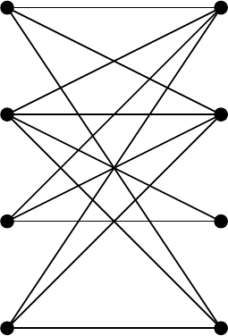
of (7.8) are illustrated in Fig. 7.2.

q =1

˜w

= −2

˜w

Fig. 7.2. Dual variables and reduced weights for G(A) (Example 7.1.11, k =3)

According to (7.13) we have the tight coeﬃcient matrix

T (A; p, q)=A

∗

⎛

⎜

⎝

••

• α 102

• 1110

• 11−10

2001

⎞

⎟

⎠

, (7.21)

which should be compared with A

◦

of (7.4); A

∗

contains a smaller number of

nonzero entries. The symbol • denotes active rows and columns. The graph

∗

consisting of the tight arcs is shown in Fig. 7.3. Noting I

∗

(p)={r

∗

(p)={c

}, we see that the conditions (R1)–(R3) in Theorem 7.1.9 are

satisﬁed for all values of α. On the other hand, the last condition (R4) is

violated when α = 1. Hence by Theorem 7.1.9 we see

(A)



(A) = 13 if α =1

≤

(A) − 1 = 12 if α =1.