Murota K. Matrices and Matroids for Systems Analysis
Подождите немного. Документ загружается.

Contents XI
4.8 Partitioned Matrix . . . . . . . . . . . . . . . . . . . . . . . . . . . . . . . . . . . . . 230
4.8.1 Definitions . . . . . . . . . . . . . . . . . . . . . . . . . . . . . . . . . . . . . . 231
4.8.2 Existence of Proper Block-triangularization . . . . . . . . . . 235
4.8.3 Partial Order Among Blocks . . . . . . . . . . . . . . . . . . . . . . . 238
4.8.4 Generic Partitioned Matrix . . . . . . . . . . . . . . . . . . . . . . . . 240
4.9 Principal Structures of LM-matrices . . . . . . . . . . . . . . . . . . . . . . 250
4.9.1 Motivations . . . . . . . . . . . . . . . . . . . . . . . . . . . . . . . . . . . . . . 250
4.9.2 Principal Structure of Submodular Systems . . . . . . . . . . 252
4.9.3 Principal Structure of Generic Matrices . . . . . . . . . . . . . 254
4.9.4 Vertical Principal Structure of LM-matrices . . . . . . . . . . 257
4.9.5 Horizontal Principal Structure of LM-matrices . . . . . . . 261
5. Polynomial Matrix and Valuated Matroid ................ 271
5.1 Polynomial/Rational Matrix . . . . . . . . . . . . . . . . . . . . . . . . . . . . . 271
5.1.1 Polynomial Matrix and Smith Form . . . . . . . . . . . . . . . . 271
5.1.2 Rational Matrix and Smith–McMillan Form at Infinity 272
5.1.3 Matrix Pencil and Kronecker Form . . . . . . . . . . . . . . . . . 275
5.2 ValuatedMatroid ...................................... 280
5.2.1 Introduction . . . . . . . . . . . . . . . . . . . . . . . . . . . . . . . . . . . . . 280
5.2.2 Examples . . . . . . . . . . . . . . . . . . . . . . . . . . . . . . . . . . . . . . . 281
5.2.3 Basic Operations . . . . . . . . . . . . . . . . . . . . . . . . . . . . . . . . . 282
5.2.4 Greedy Algorithms . . . . . . . . . . . . . . . . . . . . . . . . . . . . . . . 285
5.2.5 Valuated Bimatroid . . . . . . . . . . . . . . . . . . . . . . . . . . . . . . . 287
5.2.6 Induction Through Bipartite Graphs . . . . . . . . . . . . . . . . 290
5.2.7 Characterizations . . . . . . . . . . . . . . . . . . . . . . . . . . . . . . . . . 295
5.2.8 Further Exchange Properties . . . . . . . . . . . . . . . . . . . . . . . 300
5.2.9 Valuated Independent Assignment Problem . . . . . . . . . . 306
5.2.10 Optimality Criteria . . . . . . . . . . . . . . . . . . . . . . . . . . . . . . . 308
5.2.11 Application to Triple Matrix Product . . . . . . . . . . . . . . . 316
5.2.12 Cycle-canceling Algorithms . . . . . . . . . . . . . . . . . . . . . . . . 317
5.2.13 Augmenting Algorithms . . . . . . . . . . . . . . . . . . . . . . . . . . . 325
6. Theory and Application of Mixed Polynomial Matrices ... 331
6.1 Descriptions of Dynamical Systems . . . . . . . . . . . . . . . . . . . . . . . 331
6.1.1 Mixed Polynomial Matrix Descriptions . . . . . . . . . . . . . . 331
6.1.2 Relationship to Other Descriptions . . . . . . . . . . . . . . . . . 332
6.2 Degree of Determinant of Mixed Polynomial Matrices . . . . . . . 335
6.2.1 Introduction . . . . . . . . . . . . . . . . . . . . . . . . . . . . . . . . . . . . . 335
6.2.2 Graph-theoretic Method . . . . . . . . . . . . . . . . . . . . . . . . . . . 336
6.2.3 Basic Identities . . . . . . . . . . . . . . . . . . . . . . . . . . . . . . . . . . 337
6.2.4 Reduction to Valuated Independent Assignment . . . . . . 340
6.2.5 Duality Theorems . . . . . . . . . . . . . . . . . . . . . . . . . . . . . . . . 343
6.2.6 Algorithm . . . . . . . . . . . . . . . . . . . . . . . . . . . . . . . . . . . . . . . 348
6.3 Smith Form of Mixed Polynomial Matrices . . . . . . . . . . . . . . . . 355
6.3.1 Expression of Invariant Factors . . . . . . . . . . . . . . . . . . . . . 355
XII Contents
6.3.2 Proofs . . . . . . . . . . . . . . . . . . . . . . . . . . . . . . . . . . . . . . . . . . 363
6.4 Controllability of Dynamical Systems . . . . . . . . . . . . . . . . . . . . . 364
6.4.1 Controllability . . . . . . . . . . . . . . . . . . . . . . . . . . . . . . . . . . . 364
6.4.2 Structural Controllability . . . . . . . . . . . . . . . . . . . . . . . . . . 365
6.4.3 Mixed Polynomial Matrix Formulation . . . . . . . . . . . . . . 372
6.4.4 Algorithm . . . . . . . . . . . . . . . . . . . . . . . . . . . . . . . . . . . . . . . 375
6.4.5 Examples . . . . . . . . . . . . . . . . . . . . . . . . . . . . . . . . . . . . . . . 379
6.5 Fixed Modes of Decentralized Systems . . . . . . . . . . . . . . . . . . . . 384
6.5.1 Fixed Modes . . . . . . . . . . . . . . . . . . . . . . . . . . . . . . . . . . . . . 384
6.5.2 Structurally Fixed Modes . . . . . . . . . . . . . . . . . . . . . . . . . 387
6.5.3 Mixed Polynomial Matrix Formulation . . . . . . . . . . . . . . 390
6.5.4 Algorithm . . . . . . . . . . . . . . . . . . . . . . . . . . . . . . . . . . . . . . . 395
6.5.5 Examples . . . . . . . . . . . . . . . . . . . . . . . . . . . . . . . . . . . . . . . 398
7. Further Topics ............................................ 403
7.1 Combinatorial Relaxation Algorithm . . . . . . . . . . . . . . . . . . . . . . 403
7.1.1 Outline of the Algorithm . . . . . . . . . . . . . . . . . . . . . . . . . . 403
7.1.2 Test for Upper-tightness . . . . . . . . . . . . . . . . . . . . . . . . . . . 407
7.1.3 Transformation Towards Upper-tightness . . . . . . . . . . . . 413
7.1.4 Algorithm Description . . . . . . . . . . . . . . . . . . . . . . . . . . . . 417
7.2 Combinatorial System Theory . . . . . . . . . . . . . . . . . . . . . . . . . . . . 418
7.2.1 Definition of Combinatorial Dynamical Systems . . . . . . 419
7.2.2 Power Products . . . . . . . . . . . . . . . . . . . . . . . . . . . . . . . . . . 420
7.2.3 Eigensets and Recurrent Sets . . . . . . . . . . . . . . . . . . . . . . 422
7.2.4 Controllability of Combinatorial Dynamical Systems . . 426
7.3 Mixed Skew-symmetric Matrix . . . . . . . . . . . . . . . . . . . . . . . . . . . 431
7.3.1 Introduction . . . . . . . . . . . . . . . . . . . . . . . . . . . . . . . . . . . . . 431
7.3.2 Skew-symmetric Matrix . . . . . . . . . . . . . . . . . . . . . . . . . . . 433
7.3.3 Delta-matroid . . . . . . . . . . . . . . . . . . . . . . . . . . . . . . . . . . . . 438
7.3.4 Rank of Mixed Skew-symmetric Matrices . . . . . . . . . . . . 444
7.3.5 Electrical Network Containing Gyrators . . . . . . . . . . . . . 446
References .................................................... 453
Notation Table ............................................... 469
Index ......................................................... 479

1. Introduction to Structural Approach —
Overview of the Book
This chapter is a brief introduction to the central ideas of the combinatorial
method of this book for the structural analysis of engineering systems. We
explain the motivations and the general framework by referring, as a specific
example, to the problem of computing the index of a system of differential-
algebraic equations (DAEs). In this approach, engineering systems are de-
scribed by mixed polynomial matrices. A kind of dimensional analysis is also
invoked. It is emphasized that relevant physical observations are crucial to
successful mathematical modeling for structural analysis. Though the DAE-
index problem is considered as an example, the methodology introduced here
is more general in scope and is applied to other problems in subsequent chap-
ters.
1.1 Structural Approach to Index of DAE
1.1.1 Index of Differential-algebraic Equations
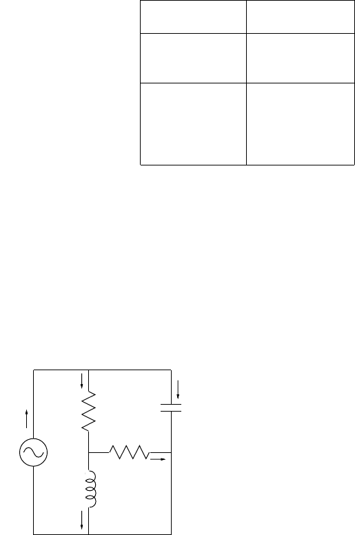
Let us start with a simple electrical network
1
of Fig. 1.1 to introduce the
concept of an index of a system of differential-algebraic equations (DAEs)
and to explain a graph-theoretic method.
The network consists of a voltage source V (branch 1), two ohmic resistors
R
1
and R
2
(branch 2 and branch 3), an inductor L (branch 4), and a capacitor
C (branch 5). A state of this network is described by a 10 dimensional vector
x =(ξ
1
, ···,ξ
5
,η
1
, ···,η
5
)
T
representing currents ξ
i
in and the voltage η
i
across branch i (i =1, ···, 5) with reference to the directions indicated in
Fig. 1.1. The governing equations in the frequency domain are given by a
system of equations A
(1)
x = b, where b =(0, 0, 0, 0, 0; V,0, 0, 0, 0)
T
is another
10 dimensional vector representing the source, and A
(1)
is a 10 × 10 matrix
defined by
1
This example, described in Cellier [28, §3.7], was communicated to the author
by P. Bujakiewicz, F. Cellier, and R. Huber.
K. Murota, Matrices and Matroids for Systems Analysis,
Algorithms and Combinatorics 20, DOI 10.1007/978-3-642-03994-2
1,
c
Springer-Verlag Berlin Heidelberg 2010
2 1. Introduction to Structural Approach — Overview of the Book
A
(1)
=
ξ
1
ξ
2
ξ
3
ξ
4
ξ
5
η
1
η
2
η
3
η
4
η
5
1 −10 0−1
−10 1 1 1
−10 0 0−1
0110−1
00−11 0
00000−10 0 0 0
0 R
1
0000 −10 0 0
00R
2
0000−10 0
000sL 0 000−10
0000−1 0000sC
. (1.1)
As usual, s is the variable for the Laplace transformation that corresponds
to d/dt, the differentiation with respect to time (see Remark 1.1.1 for the
Laplace transformation). The first two equations, corresponding to the 1st
and 2nd rows of A
(1)
, represent Kirchhoff ’s current law (KCL), while the
following three equations Kirchhoff’s voltage law (KVL). The last five equa-
tions express the element characteristics (constitutive equations). The system
of equations, A
(1)
x = b, represents a mixture of differential equations and
algebraic equations (i.e., a linear time-invariant DAE), since the coefficient
matrix A
(1)
contains the variable s.
V
L
R
1
R
C
2
2
5
3
1
4
Fig. 1.1. An electrical network
For a linear time-invariant DAE in general, say Ax = b with A = A(s)
being a nonsingular polynomial matrix in s,theindex is defined (see Remark
1.1.2) by
ν(A) = max
i,j
deg
s
(A
−1
)
ji
+1. (1.2)
Here it should be clear that each entry (A
−1
)
ji
of A
−1
is a rational function in
s and the degree of a rational function p/q (with p and q being polynomials)
is defined by deg
s
(p/q) = deg
s
p −deg
s
q. An alternative expression for ν(A)
is
1.1 Structural Approach to Index of DAE 3
ν(A) = max
i,j
deg
s
((i, j)-cofactor of A) − deg
s
det A +1. (1.3)
For the matrix A
(1)
of (1.1), we see
max
i,j
deg
s
((i, j)-cofactor of A
(1)
) = deg
s
((6, 5)-cofactor of A
(1)
)=2,
det A
(1)
= R
1
R
2
+ sL · R
1
+ sL · R
2
(1.4)
by direct calculation and therefore ν(A
(1)
)=2− 1 + 1 = 2 by the formula
(1.3).
The solution to Ax = b is of course given by x = A
−1
b, and therefore
ν(A) − 1 equals the highest order of the derivatives of the input b that can
possibly appear in the solution x. As such, a high index indicates difficulty
in the numerical solution of the DAE, and sometimes even inadequacy in
the mathematical modeling. Note that the index is equal to one for a system
of purely algebraic equations (where A(s) is free from s), and to zero for a
system of ordinary differential equations in the normal form (dx/dt = A
0
x
with a constant matrix A
0
, represented by A(s)=sI − A
0
).
Remark 1.1.1. For a function x(t), t ∈ [0, ∞), the Laplace transform is
defined by ˆx(s)=
∞
0
x(t)e
−st
dt, s ∈ C. The Laplace transform of dx(t)/dt
is given by sˆx(s)ifx(0) = 0. See Doetsch [49] and Widder [341] for precise
mathematical accounts and Chen [33], Kailath [152] and Zadeh–Desoer [350]
for system theoretic aspects of the Laplace transformation. 2
Remark 1.1.2. The definition of the index given in (1.2) applies only to
linear time-invariant DAE systems. An index can be defined for more general
systems and two kinds are distinguished in the literature, a differential index
and a perturbation index, which coincide with each other for linear time-
invariant DAE systems. See Brenan–Campbell–Petzold [21], Hairer–Lubich–
Roche [100], and Hairer–Wanner [101] for details. 2
Remark 1.1.3. Extensive study has been made recently on the DAE in-
dex in the literature of numerical computation and system modeling. See,
e.g., Brenan–Campbell–Petzold [21], Bujakiewicz [26], Bujakiewicz–van den
Bosch [27], Cellier–Elmqvist [29], Duff–Gear [60], Elmqvist–Otter–Cellier
[72], Gani–Cameron [86], Gear [88, 89], G¨unther–Feldmann [98], G¨unther–
Rentrop [99], Hairer–Wanner [101], Mattsson–S¨oderlind [188], Pantelides
[264], Ponton–Gawthrop [272], and Ungar–Kr¨oner–Marquardt [324]. 2
1.1.2 Graph-theoretic Structural Approach
Structural considerations turn out to be useful in computing the index of
DAE. This section describes the basic idea of the graph-theoretic structural
methods.
In the graph-theoretic structural approach we extract the information
about the degree of the entries of the matrix, ignoring the numerical values

4 1. Introduction to Structural Approach — Overview of the Book
of the coefficients. Associated with the matrix A
(1)
of (1.1), for example, we
consider
A
(1)
str
=
ξ
1
ξ
2
ξ
3
ξ
4
ξ
5
η
1
η
2
η
3
η
4
η
5
t
1
t
2
00t
3
t
4
0 t
5
t
6
t
7
t
8
000 t
9
0 t
10
t
11
0 t
12
00t
13
t
14
0
00000t
15
000 0
0 t
16
0000 t
17
00 0
00t
18
0000t
19
00
00 0st
20
0 000t
21
0
00 0 0 t
22
0000st
23
where t
1
, ···,t
23
are assumed to be independent parameters.
For a polynomial matrix A = A(s)=(A
ij
) in general, we consider a
matrix A
str
= A
str
(s), called the structured matrix associated with A,in
a similar manner. For a nonzero entry A
ij
,letα
ij
s
w
ij
be its leading term,
where α
ij
∈ R \{0} and w
ij
= deg
s
A
ij
. Then (A
str
)
ij
is defined to be
equal to s
w
ij
multiplied by an independent parameter t
ij
. Note that the
numerical information about the leading coefficient α
ij
is discarded with the
replacement by t
ij
. Namely, we define the (i, j)entryofA
str
by
(A
str
)
ij
=
t
ij
s
deg
s
A
ij
(if A
ij
=0)
0 (if A
ij
=0)
(1.5)
where t
ij
is an independent parameter. We refer to the index of A
str
in the
sense of (1.2) or (1.3) as the structural index of A and denote it by ν
str
(A),
namely,
ν
str
(A)=ν(A
str
). (1.6)
Two different matrices, say A and A
, are associated with the same struc-
tured matrix, A
str
= A
str
, if deg
s
A
ij
= deg
s
A
ij
for all (i, j). In other words,
a structured matrix is associated with a family of matrices that have a com-
mon structure with respect to the degrees of the entries. Though there is
no guarantee that the structural index ν
str
(A) coincides with the true in-
dex ν(A) for a particular (numerically specified) matrix A,itistruethat
ν
str
(A
)=ν(A
) for “almost all” matrices A
that have the same structure
as A in the sense of A
str
= A
str
. That is, the equality ν
str
(A
)=ν(A
) holds
true for “almost all” values of t
ij
’s, or, in mathematical terms, “generically”
with respect to the parameter set {t
ij
| A
ij
=0}. (The precise definition of
“generically” is given in §2.1.)
The structural index has the advantage that it can be computed by an
efficient combinatorial algorithm free from numerical difficulties. This is based
on a close relationship between subdeterminants of a structured matrix and
matchings in a bipartite graph.
1.1 Structural Approach to Index of DAE 5
Specifically, we consider a bipartite graph G(A)=(Row(A), Col(A); E)
with the left vertex set corresponding to the row set Row(A) of the matrix
A, the right vertex set corresponding to the column set Col(A), and the edge
set corresponding to the set of nonzero entries of A =(A
ij
), i.e.,
E = {(i, j) | i ∈ Row(A),j ∈ Col(A),A
ij
=0}.
Each edge (i, j) ∈ E is given a weight w
ij
= deg
s
A
ij
.
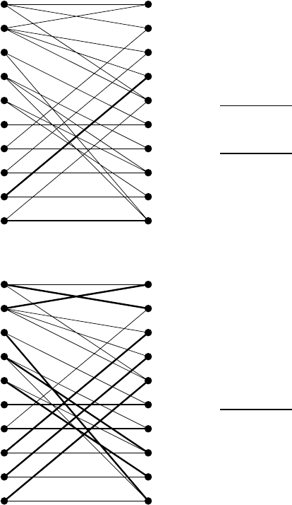
For instance, the bipartite graph G(A
(1)
) associated with our example
matrix A
(1)
of (1.1) is given in Fig. 1.2(a). The thin lines indicate edges
(i, j) of weight w
ij
= 0 and the thick lines designate two edges, (i, j)=
(9, 4), (10, 10), of weight w
ij
=1.
A matching M in G(A) is, by definition, a set of edges (i.e. M ⊆ E) such
that no two members of M have an end-vertex in common. The weight of
M, denoted w(M), is defined by
w(M)=
(i,j)∈M
w
ij
,
while the size of M means |M|, the number of edges contained in M.We
denote by M
k
the family of all the matchings of size k in G(A)fork =1, 2, ···,
and by M the family of all the matchings of any size (i.e., M = ∪
k
M
k
).
For example, the thick lines in Fig. 1.2(b) show a matching M of weight
w(M) = 1 and of size |M| = 10, and M
=(M \{(3, 10), (10, 5)}) ∪{(10, 10)}
is a matching of weight w(M
) = 2 and of size |M
| =9.
Assuming that A
str
is an n×n matrix, we consider the defining expansion
of its determinant:
det A
str
=
π∈S
n
sgn π ·
n
i=1
(A
str
)
iπ(i)
=
π∈S
n
sgn π ·
n
i=1
t
iπ(i)
· s
n
i=1
w
iπ(i)
,
where S
n
denotes the set of all the permutations of order n, and sgn π = ±1
is the signature of a permutation π. We observe the following facts:
1. Nonzero terms in this expansion correspond to matchings of size n in
G(A);
2. There is no cancellation among different nonzero terms in this expansion
by virtue of the independence among t
ij
’s.
These two facts imply the following:
1. The structured matrix A
str
is nonsingular (i.e., det A
str
= 0) if and only
if there exists a matching of size n in G(A);
2. In the case of a nonsingular A
str
,itholdsthat
deg
s
det A
str
= max
M
n
∈M
n
w(M
n
). (1.7)
6 1. Introduction to Structural Approach — Overview of the Book
Rows
1
2
3
4
5
6
7
8
9
10
Columns
1
2
3
4
5
6
7
8
9
10
weight=0
weight=1
(a)
Rows
1
2
3
4
5
6
7
8
9
10
Columns
1
2
3
4
5
6
7
8
9
10
maximum-weight
matching of size 10
(weight = 1)
(b)
Fig. 1.2. Graph G(A
(1)
) and the maximum-weight matching
A similar argument applied to submatrices of A
str
leads to more general
formulas:
rank A
str
= max
M∈M
|M|,
max
|I|=|J|=k
deg
s
det A
str
[I,J] = max
M
k
∈M
k
w(M
k
)(k =1, ···,r
str
), (1.8)
where A
str
[I,J] means the submatrix of A
str
having row set I and column
set J,andr
str
=rankA
str
. It should be clear that the left-hand side of (1.8)
designates the maximum degree of a minor (subdeterminant) of order k.
1.1 Structural Approach to Index of DAE 7
A combination of the formulas (1.3) and (1.8) yields
ν
str
(A) = max
M
n−1
∈M
n−1
w(M
n−1
) − max
M
n
∈M
n
w(M
n
) + 1 (1.9)
for a nonsingular n × n polynomial matrix A.Thuswehavearrivedata
combinatorial expression of the structural index.
For the matrix A
(1)
we have (cf. Fig. 1.2)
max
M
(1)
n−1
∈M
(1)
n−1
w(M
(1)
n−1
)=2, max
M
(1)
n
∈M
(1)
n
w(M
(1)
n
)=1
and therefore ν
str
(A
(1)
)=2− 1 + 1 = 2, in agreement with ν(A
(1)
)=2.
It is important from the computational point of view that efficient combi-
natorial algorithms are available for checking the existence of a matching of a
specified size and also for finding a maximum-weight matching of a specified
size. Thus the structural index ν
str
, with the expression (1.9), can be com-
puted efficiently by solving weighted bipartite matching problems utilizing
those efficient combinatorial algorithms.
A number of graph-theoretic techniques (which may be considered vari-
ants of the above idea) have been proposed as “structural algorithms” (Bu-
jakiewicz [26], Bujakiewicz–van den Bosch [27], Duff–Gear [60], Pantelides
[264], Ungar–Kr¨oner–Marquardt [324]). It is accepted that structural consid-
erations should be useful and effective in practice for the DAE-index problem
and that the generic values computed by graph-theoretic “structural algo-
rithms” have practical significance.
1.1.3 An Embarrassing Phenomenon
While the structural approach is accepted fairly favorably, its limitation has
also been realized in the literature. A graph-theoretic structural algorithm, ig-
noring numerical data, may well fail to render the correct answer if numerical
cancellations do occur for some reason or other. So the failure of a graph-
theoretic algorithm itself should not be a surprise. The aim of this section is
to demonstrate a further embarrassing phenomenon that the structural index
of our electrical network varies with how KVL is described.
Recall first that the 3rd row of the matrix A
(1)
represents the conservation
of voltage along the loop 1–5 (V –C). In place of this we now take another
loop 1–2–4 (V –R
1
–L) to obtain a second description of the same electrical
network. The coefficient matrix of the second description is given by

8 1. Introduction to Structural Approach — Overview of the Book
A
(2)
=
ξ
1
ξ
2
ξ
3
ξ
4
ξ
5
η
1
η
2
η
3
η
4
η
5
1 −10 0−1
−10 1 1 1
−1 −10−10
0110−1
00−11 0
00000−10 0 0 0
0 R
1
0000 −10 0 0
00R
2
0000−10 0
000sL 0 000−10
0000−1 0000sC
, (1.10)
which differs from A
(1)
in the 3rd row. The associated structured matrix A
(2)
str
differs from A
(1)
str
also in the 3rd row, and is given by
A
(2)
str
=
ξ
1
ξ
2
ξ
3
ξ
4
ξ
5
η
1
η
2
η
3
η
4
η
5
t
1
t
2
00t
3
t
4
0 t
5
t
6
t
7
t
24
t
25
0 t
26
0
0 t
10
t
11
0 t
12
00t
13
t
14
0
00 0 0 0t
15
000 0
0 t
16
0000 t
17
00 0
00t
18
0000t
19
00
00 0st
20
0 000t
21
0
00 0 0 t
22
0000st
23
,
where {t
i
| i =1, ···, 7, 10, ···, 26} is the set of independent parameters.
Naturally, the index should remain invariant against this trivial change
in the description of KVL, and in fact we have
ν(A
(1)
)=ν(A
(2)
)=2.
It turns out, however, that the structural index does change, namely,
ν
str
(A
(1)
)=2,ν
str
(A
(2)
)=1,
where the latter is computed from the graph G(A
(2)
) in Fig. 1.3; we have
max
M
(2)
n−1
∈M
(2)
n−1
w(M
(2)
n−1
)=2, max
M
(2)
n
∈M
(2)
n
w(M
(2)
n
)=2
and therefore
ν
str
(A
(2)
)=ν(A
(2)
str
)=2− 2+1=1
according to the expression (1.9).
The discrepancy between the structural index ν
str
(A
(2)
) and the true in-
dex ν(A
(2)
) is ascribed to the discrepancy between deg
s
det A
(2)
str
=2and