Mikles J., Fikar M. Process Modelling, Identification, and Control

260 7 The Control Problem and Design of Simple Controllers

• f

= e(t) : (IE = integral of error) is the simplest function. The advan-

tage are simple calculations. However, it is only suitable for overdamped

transient responses as otherwise positive and negative parts cancel them-

selves and the criterion can be zero even if the transient response is highly

oscillatory.

• f

= |e(t)| : (IAE = integral absolute value of error) removes the drawback

of the previous approach and is also suitable for oscillatory responses. How-

ever, from the computational point of view, it can be diﬃcult to implement

as the absolute value is non-diﬀerentiable.

• f

= |e(t)|t : (ITAE = integral time multiplied absolute value of error)

the time term in the cost function penalises the settling time, as well as

reduces the large initial error in the cost function. Otherwise it is the same

as the previous one.

• f

= e

(t) : (ISE = integral squared value of error) combines advantages of

a simple surface and of the absolute value. Large values of control error are

penalised more than small values and lead to controllers with larger settling

time than the IAE cost. Squared error is mathematically convenient for

analytical purposes.

• f

= e

(t)t : improves the previous cost and decreases the settling time.

• f

= e

(t)+φ ˙e

(t) : by penalising a square of derivative suppresses oscilla-

tory behaviour typical for ISE cost. Dampens large changes of the control

error and thus also large values of the manipulated input and its change.

The choice of the penalisation factor φ can be diﬃcult.

• f

= e

(t)+φu

(t) : can suitably penalise the manipulated variable and

simply regulate the ratio between speed and robustness of the controller.

In each case it has been assumed that e(t)andu(t) are stable and con-

verge to zero, so that the cost functions converge. If this is not correct, it is

necessary to work with deviations of the variables from their steady state or

to implement some special strategy.

7.3.3 Control Quality and Frequency Indices

Control quality can also be characterised by frequency domain indices. Some

of them measure directly quality, others describe relative stability,i.e.quantify

how far is the closed-loop system away from instability.

• Gain margin measures relative stability and is deﬁned as the amount of

gain that can be inserted in the loop before the closed-loop system reaches

instability. Mathematically spoken it is the magnitude of the reciprocal of

the open-loop transfer function evaluated at the frequency ω

at which

the phase angle of the frequency transfer function is −180

◦

GM =

(ω

(7.20)

7.3 Control Performance Indices 261

where arg G

(ω

)=−180

◦

= −π and ω

is called the phase crossover

frequency.

• Phase margin is a measure of relative stability and it is deﬁned as 180

◦

plus

the phase angle of the open-loop at the frequency ω

at unity open-loop

gain

= 180

◦

+ ϕ[G

(ω

)] (7.21)

where |G

(ω

)| =1andω

is called the gain crossover frequency. Recom-

mended values are between 30

◦

− 65

◦

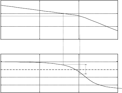
Gain and phase margins are graphically shown in Bode plots in Fig. 7.5.

-1

-100

-50

Magnitude

[dB]

-1

-300

-250

-200

-150

-100

-50

Frequency [rad/min]

Phase

[deg]

1/PM

Fig. 7.5. Gain and phase margins for a typical continuous system. Intersection for

is at the value 0 dB

• Bandwidth ω

. Loosely spoken it is deﬁned as the frequency range over

which the system responds satisfactorily. Often it is deﬁned as the fre-

quency range where the magnitude is approximately constant compared

to the value at some speciﬁed frequency and diﬀers by not more than

−3 dB. However, there are also other deﬁnitions. A good approximation is

the frequency ω

deﬁned by (7.21).

• Cutoﬀ rate is the frequency rate at which the magnitude decreases beyond

the cutoﬀ frequency ω

. For example it can be chosen as 6 dB / decade.

• Resonance peak M

is the maximum of the magnitude frequency response.

• Resonant frequency ω

is the frequency at which the resonance peak oc-

curs.

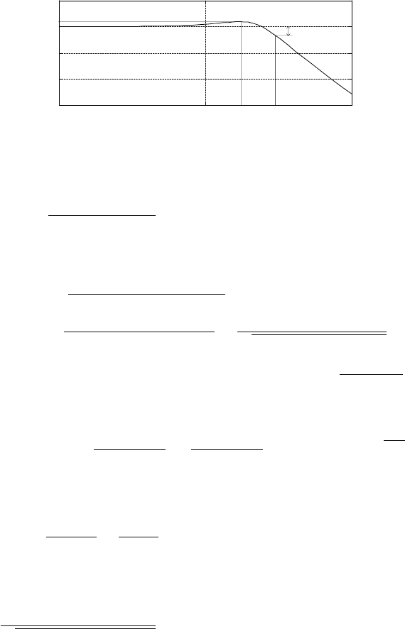
These indices are shown in Fig. 7.6.

Example 7.2: Gain and phase margins

Let us consider a system with the transfer function

262 7 The Control Problem and Design of Simple Controllers

-1

-30

-20

-10

Frequency [rad/min]

Magnitude [dB]

3 dB

Fig. 7.6. Bandwidth, resonant peak, and resonance frequency in magnitude fre-

quency response

G(s)=

432

s(s

+13s + 115)

Substituting s =jω, the magnitude and phase of the transfer function is

given as

|G(jω)| =



432

(jω)

+ 13(jω)

+ 115(jω)



432

|−13ω

+ j(115ω − ω

432



169ω

+ (115ω − ω

)

ϕ = ϕ(1) − ϕ(−13ω

+ j(115ω − ω

)) = −arctan

115ω − ω

13ω

To ﬁnd the gain margin it is necessary to determine the frequency when

the phase is equal to ϕ = −π. This gives

−π = −arctan

115ω

− ω

13ω

⇒

115ω

− ω

13ω

= tan π ⇒ ω

√

115

Gain margin is given by the reciprocal of the magnitude of the transfer

function at this frequency (7.20), hence

GM =

|G(jω

0.2897

=3.45

For phase margin it is necessary to ﬁnd the frequency when the magnitude

is equal to one

432



169ω

+ (115ω

− ω

)

Manipulating this equation yields the 6th order equation

− 61ω

+ 115

− 432

Solving this equation gives a single real positive root ω

=3.858. From

the phase at this frequency follows from (7.21) φ

=63

◦

Fig. 7.5 illustrates graphical procedure to ﬁnd the indices for this system.

7.3 Control Performance Indices 263

Example 7.3: Determination of the resonant peak

Consider a system with the transfer function

G(s)=

+2s +5

We will ﬁnd values of the resonant peak M

, the corresponding resonance

frequency ω

, and bandwidth ω

. As these are calculated from the mag-

nitude frequency resonance, this will be derived at ﬁrst

|G(jω)| =

|−ω

+2jω +5|

√

− 6ω

+25

The maximum can be found by setting the derivative equal to zero

(ω

− 3) = 0

Only the second root has meaning and thus ω

√

3. The resonant peak

is then

= |G(jω

)| =

− 6ω

+25

=1.25

Bandwidth can be determined if the magnitude of G(s) decreases by 3 dB

as compared to the value at the beginning (0.707G(0)). As G(0) = 1, it

holds

|G(jω

)| =

√

⇒ ω

=2.97.

Fig. 7.6 illustrates graphical procedure to ﬁnd the indices.

7.3.4 Poles

Very often speciﬁcation of the control quality can be described by the locations

of poles. Of course, stability dictates the left half plane for the pole locations.

A suitable pole region is shown in Fig. 7.7.

In general, the closer the pole is near the origin, the larger settling time

results. A real pole is coupled with aperiodic (overdamped) response. If the

closed-loop system has more poles, some of them dominate the process dy-

namics – the so called dominant poles. These poles are at least ﬁve times

nearer to the origin as the other. This means that for example when designing

a pole placement control design it is necessary to characterise only 2-3 poles

and the rest needed for physical realisation of the controller can be chosen

within the far left half plane.

To clarify the relations and inﬂuences among several speciﬁcations let us

consider the following example.

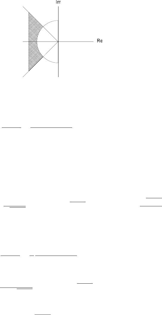
264 7 The Control Problem and Design of Simple Controllers

Fig. 7.7. Suitable region for pole locations of a closed-loop system

Example 7.4: A second order system - quality indices

Let us consider a closed-loop system with the transfer function of the form

1+GR

+2ζω

s + ω

(7.22)

where ζ is the damping coeﬃcient and ω

is the natural undamped

frequency. This transfer function can be obtained with a ﬁrst order con-

trolled system with gain Z and time constant T controlled by a controller

with the transfer function R =1/T

s. In that case holds ω

= Z/TT

2ζω

=1/T .

Assume that the damping coeﬃcient is inside ζ ∈ (0, 1). If the setpoint is

the unit step change then the controlled output is given as

y(t)=1−



1 −ζ

−ζω

sin





1 −ζ

+ ϕ



,ϕ= arctan



1 −ζ

(7.23)

Similarly, the transfer function between the output and a disturbance

acting on the plant input is given as

1+GR

+2ζω

s + ω

(7.24)

and the time response for the unit step change of the disturbance is

e(t)=



1 −ζ

−ζω

sin





1 −ζ



(7.25)

The closed-loop poles are complex conjugated and of the form

1,2

= −ζω

± jω



1 −ζ

(7.26)

7.3 Control Performance Indices 265

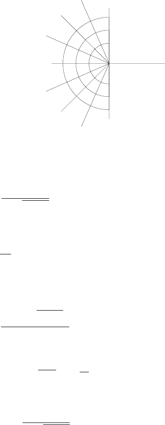
When the frequency ω

is assumed constant then poles are located in the

complex plane on half circles with radius ω

centered in origin. If ζ is

constant, then half lines from origin occur with slope being a function of

ζ (Fig. 7.8).

Fig. 7.8. Curves with constant values of ζ,ω

(ζ

<ζ

, ω

<ω

)

The process is underdamped with a period

2π



1 −ζ

(7.27)

and damping coeﬃcient

ϕ/ tan ϕ

(7.28)

Settling time T



for a band with accuracy ±p from the steady state is a

complex function of parameters, but can be approximated as



≈

log





1 −ζ



ζω

(7.29)

Maximum overshoot is given by the relation

max

−πζ

√

1−ζ



(7.30)

and occurs at the time

t(e

max



1 −ζ

(7.31)

If a step change of a disturbance at the plant input is considered, then for

its maximum value holds

266 7 The Control Problem and Design of Simple Controllers

max

Tω



1 −ζ

ϕ tan ϕ

sin ϕ (7.32)

t(e

max



1 −ζ

ϕ (7.33)

and the integral performance index IE can be derived as

(7.34)

These expressions can be used for better understanding of performance

indices and their relations to controller parameters and vice versa. Integral

cost function value is inversely proportional to ω

. Maximum overshoot

and all time indices are inversely proportional to ω

. Transient response

of the closed-loop system to setpoints or disturbances is improved by in-

creasing ω

. Further, maximum overshoot or damping coeﬃcient increase

with decreasing ζ.

Results presented in the example do not hold only for closed-loop systems

with the given transfer function but can also be generalised for other systems

as almost any process can be decomposed into a set of the ﬁrst and second

order systems. Moreover, from the dynamic point of view, in the majority of

processes some subsystem dominates over the rest and the overall system is

approximable by a second order system.

7.4 PID Controller

Among various controllers used in industry, the PID (proportional-integral-

derivative) controller is the most often employed. There are estimates that

more than 90% of controllers are of PID type. Its advantage is simplicity,

robustness as well as the fact that it can be realised in various analogue

(electrical, pneumatic), as well as digital versions.

The principle of the PID controller is processing of its input signal – control

error in three branches that will be examined in more detail below.

7.4.1 Description of Components

Proportional Controller

Consider the most simple form of a feedback controller described be the ex-

pression

u(t)=



max

if e(t) > 0

min

if e(t) < 0

(7.35)

In this case the manipulated input u can have only two values depending on the

control error e sign. This controller is called on-oﬀ controller. Its advantage

7.4 PID Controller 267

is simplicity and easy implementation. As the control signal is not deﬁned

for e = 0 (see eq. (7.35)), it is usually modiﬁed by introducing some kind of

hysteresis in the neighbourhood of zero.

Its drawbacks are oscillations of the controlled variable in the steady-state

as even a small control error causes the maximum value of the manipulated

input. A suitable improvement for this situation can be introduction of pro-

portional behaviour for small control errors

u(t)=Z

e(t) (7.36)

The controller that realises this equation is called proportional (P controller)

and Z

is its gain.

From the practical point of view can any controller realise proportional

action only in some limited range of control errors as the manipulated vari-

able can always be only in the range between u

min

and u

max

. Proportional

behaviour of the controller can then be characterised either by its gain Z

by some range when the controller is linear – proportionality band P

. Their

relation is

max

− u

min

= Z

(7.37)

If we consider the maximum range of the manipulated variable normalised, e.

g. u

max

− u

min

= 100% then

100

(7.38)

If the control error is too large in magnitude then the P controller implements

on-oﬀ behaviour with the manipulated variable constrained to its maximum

and minimum values.

From steady-state analysis of the P controller (see page 256) follows that

if the controlled system does not contain at least one pure integrator, the

closed-loop system will exhibit non-zero permanent control error. The sim-

plest scheme to guarantee the zero steady-state control error is to introduce

a suitable constant term u

to the manipulated variable

u(t)=Z

e(t)+u

(t) (7.39)

such that for e(t) = 0 holds u = u

Example 7.5: Proportional control of a heat exchanger

www

Consider a feedback control of a heat exchanger with the P controller

described by the transfer function R(s)=Z

. The heat exchanger can be

given by the diﬀerential equation



+ y = Z

u +

268 7 The Control Problem and Design of Simple Controllers

where u is the manipulated variable and d is a disturbance. For the sim-

ulation purposes assume that Z

=1,T

=1.

Consider at ﬁrst the disturbance rejection case when the disturbance is a

step change. (W (s)=0,D(s)=A/s).

The closed-loop transfer function with respect to the disturbance is in this

case given as

1+GR

s+1

1+Z

s+1

The output variable is then given as

Y (s)=

s+1

1+Z

s+1

1+Z

y(t)

1+Z



1 −e

−

/(1+Z

)



The heat exchanger output is stable for any value of Z

and its new

steady-state settles at the value

y(∞)=

1+Z

A permanent control error exists

e(∞)=w(∞) − y(∞)=−

1+Z

This conﬁrms that by increasing the controller gain decreases the control

error (Fig. 7.9).

The slope of the response in time t = 0 will be derived by evaluating the

derivative

1+Z

−

/(1+Z

)



t=0

It is clear that all step responses have the same slope in time t =0

(Fig. 7.9).

Consider now tracking case when the setpoint is a step change (W (s)=

A/s, D(s) = 0).

The closed-loop transfer function with respect to the setpoint is in this

case given as

1+GR

s +1+Z

The output variable is then given as

7.4 PID Controller 269

Y (s)=

s +1+Z

1+Z

s +1

y(t)

1+Z



1 −e

−

/(1+Z

)



The heat exchanger output is stable for any value of Z

and its new

steady-state settles at the value

y(∞)=

1+Z

A permanent control error exists

e(∞)=w(∞) − y(∞)=A



1 −

1+Z



This again conﬁrms that by increasing the controller gain decreases the

control error.

The slope of the response in time t = 0 is given as

1+Z

−

/(1+Z

)



t=0

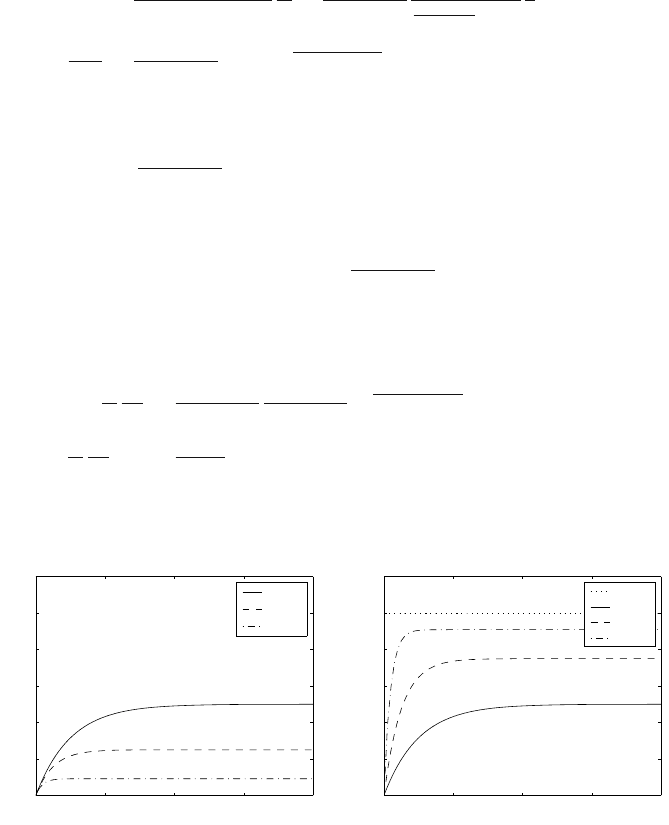
Compared to the disturbance rejection case, here the speed of the response

increases with the increasing controller gain (Fig. 7.10).

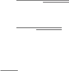
0 1 2 3 4

0.2

0.4

0.6

0.8

1.2

y/AZ

t/T

=10

Fig. 7.9. Response of a heat exchanger

to a step change of the d with a P con-

troller

0 1 2 3 4

0.2

0.4

0.6

0.8

1.2

y/A

t/T

=10

Fig. 7.10. Response of a heat exchanger

to a step change of the w with a P con-

troller

In both cases it can be noticed that the controller changes the closed-loop

time constant from the open-loop value T

to T

/(1 + Z

). If negative

feedback is assumed, both gains Z

a Z

have to be positive and the

resulting time constant is smaller than the one of the controlled system

– the closed-loop acts faster to a setpoint or disturbance changes as the

Mikles J., Fikar M. Process Modelling, Identification, and Control

Подождите немного. Документ загружается.