Middleton W.M. (ed.) Reference Data for Engineers: Radio, Electronics, Computer and Communications
Подождите немного. Документ загружается.

43-16
10
wx
00
01
11
10
YZ
00
01
11
10
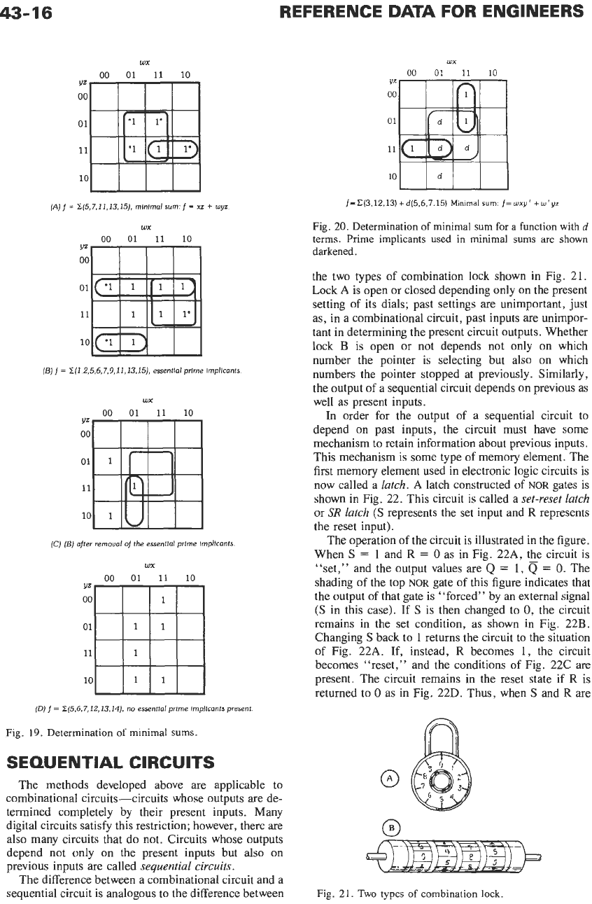
(Ajf=
~f5,7,11,13,15j,
minlmolsurn.f=
xz
+
wyz
wx
00
01
11
10
d
fBj
f
=
2(1,2,5,6,7,9,11,13,15j,
essential prime impllcents
wx
00
01
11
10
(Cj
[Bj
after removal
of
the essentlol prlrne lrnpllcants
wx
00
01
11
10
YZ
00
01
11
10
[Dj
f
=
2(5,6,7,12,13,14j,
no
essentfol prime
lrnpllcants
present
Fig.
19.
Determination
of
minimal sums.
SEQUENTIAL CIRCUITS
The methods developed above
are
applicable to
combinational circuits-circuits whose outputs are de-
termined completely by their present inputs. Many
digital circuits satisfy
this
restriction; however, there are
also many circuits that do not. Circuits whose outputs
depend not only
on
the present inputs but
also
on
previous inputs are called sequential
circuits.
The difference between a combinational circuit and a
sequential circuit is analogous to the difference between
REFERENCE
DATA
FOR ENGINEERS
WX
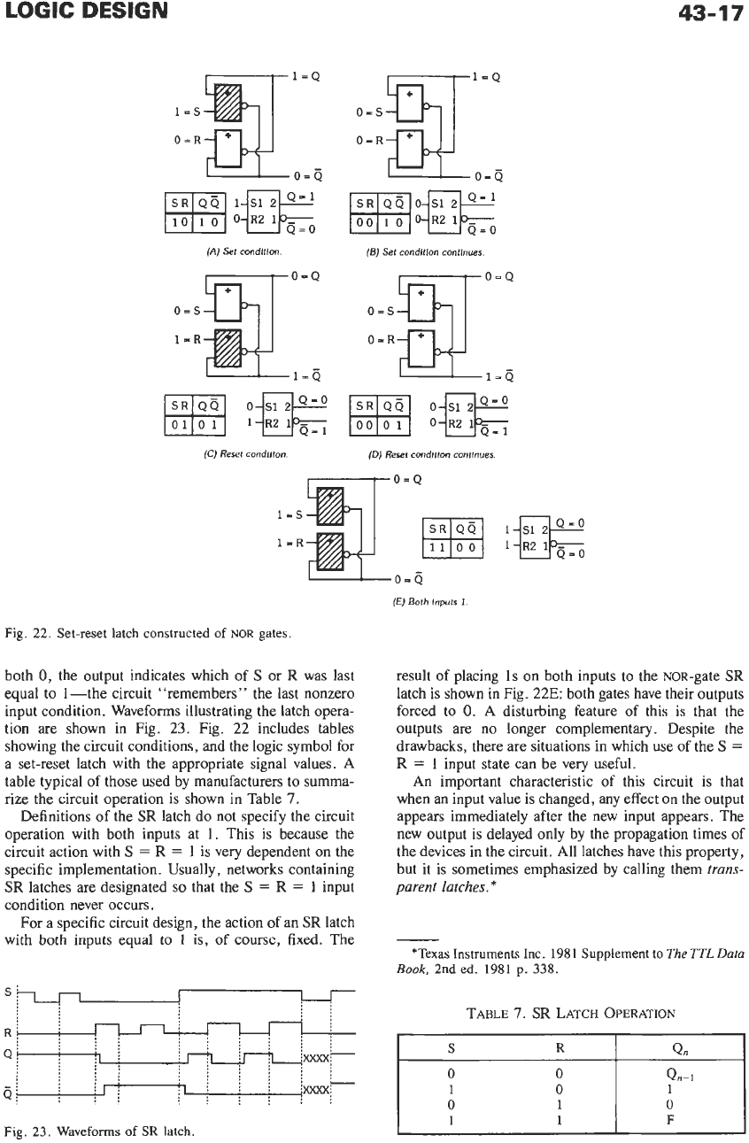
Fig.
21.
Two
types
of
combination lock.
LOGIC
DESIGN
43-17
0=6
m:wo
(A)
Set
condition
(5)
Set
condition
continues.
o=s
iD)
Reset
condltlon
contlnues
1C)
Reset
condltlon.
l=S
l=R
O=ij
(E)
Both
Inputs
1
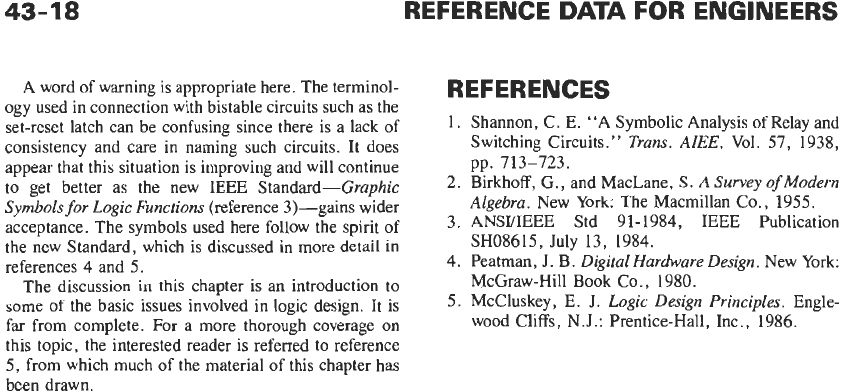
Fig.
22. Set-reset latch constructed
of
NOR
gates
both
0,
the output indicates which of
S
or
R
was last
equal to 1-the circuit “remembers” the last nonzero
input condition. Waveforms illustrating the latch opera-
tion are shown in Fig.
23.
Fig.
22
includes tables
showing the circuit conditions, and the logic symbol for
a set-reset latch with the appropriate signal values. A
table typical of those used by manufacturers to summa-
rize the circuit operation is shown in Table
7.
Definitions of the
SR
latch do not specify the circuit
operation with both inputs at 1. This is because the
circuit action with
S
=
R
=
1
is very dependent on the
specific implementation. Usually, networks containing
SR
latches
are
designated
so
that the
S
=
R
=
1 input
condition never occurs.
For
a
specific circuit design, the action of an
SR
latch
with both inputs equal to
1
is,
of
course, fixed. The
Fig.
23. Waveforms
of
SR
latch.
result
of
placing 1s on both inputs to the NOR-gate
SR
latch is shown in Fig.
22E:
both gates have their outputs
forced to
0.
A disturbing feature
of
this is that the
outputs are no longer complementary. Despite the
drawbacks, there are situations in which use of the
S
=
R
=
1
input state can be very useful.
An important characteristic of this circuit is that
when an input value is changed, any effect on the output
appears immediately after the new input appears. The
new output is delayed only by the propagation times of
the devices in the circuit. All latches have this property,
but it is sometimes emphasized by calling them
trans-
parent latches.
*
*Texas Instruments Inc. 1981 Supplement
to
The
TTL
Data
Book,
2nd ed. 1981
p.
338.
A word of warning
is
appropriate here. The terminol-
ogy used in connection with bistable circuits such as the
set-reset latch can be confusing since there is a lack
of
consistency and care in naming such circuits. It does
appear that this situation is improving and will continue
to get better as the new IEEE Standard-Graphic
Symbols
for Logic Functions (reference 3)-gains wider
acceptance. The symbols used here follow the spirit of
the new Standard, which is discussed in more detail in
references 4 and
5.
The discussion in this chapter is an introduction to
some of the basic issues involved in logic design. It is
far from complete.
For
a more thorough coverage on
this topic, the interested reader is referred to reference
5,
from which much
of
the material of this chapter has
been drawn.
REFERENCES
1. Shannon, C.
E.
“A Symbolic Analysis of Relay and
Switching Circuits.” Trans.
AIEE,
Vol.
57, 1938,
pp. 713-723.
2. Birkhoff, G., and MacLane,
S.
A
Survey
of
Modern
Algebra. New York: The Macmillan
Co.,
1955.
3. ANSUIEEE Std 91-1984, IEEE Publication
SH08615, July 13, 1984.
4. Peatman, J. B. Digital Hardware Design. New York:
McGraw-Hill
Book
Co., 1980.
5.
McCluskey, E.
J.
Logic Design Principles. Engle-
wood Cliffs, N.J.: Prentice-Hall, Inc., 1986.
44
Probability
and
Statistics
Surendra
M.
Gupta
Introduction 44-2
Discrete Probability Distribution
Continuous Probability Distribution
Mathematical Expectation
44-3
Important Theoretical Probability Distributions
44-4
Goodness
of
Fit
44-4
44-
1
44-2
REFERENCE
DATA
FOR ENGINEERS
I
NTROD
U
CTlO
N
Probability and statistics concepts have very useful
applications in science and engineering. This chapter
briefly introduces some of the important concepts of
probability and statistics.
In
probabilistic modeling one often refers to
a
ran-
dom experiment,
which represents an experiment that
can be repeated time and again under similar circum-
stances, but which yields unpredictable results at each
trial. For example, tossing
a
die is
a
random experi-
ment where the result is
a
number from the sample
space
{
1,2,3,4,5,6].
A
random experiment may con-
sist of observing or measuring elements taken from
a
set that is known
as
a
population.
A real number
asso-
ciated with the result of
a
random experiment is called
a
random variable
or
variute.
A variate may be
dis-
crete
or
continuous.
Discrete Probability
Distribution
A discrete variate takes its value from
a
finite or
denumerable set
{x,,
x2,
. .
.,
x,)
described by itsproba-
bility function,
pk,
defined
as
the probability of obtain-
ing
x,
as a
result
of
one trial.
pic
has the following
properties:
osp,
51
and
ZPk
all
k
A discrete variate can be described by its
cumulative
probability function
as
Xk5X
A
discrete variate of multiple dimensions is described
by its
joint distribution.
For example, if
(xi,
yk)
are the
coordinates of
a
point in the
(x,
y)
plane, then
p(xl,
yk)
is
the joint probability distribution such that
x
=
xj
and
y
=
yk.
In
addition,
all
k
and
P2(Yk)=xP(XJ,Yk)
all
j
are, respectively, the
marginal probabilities
that
x
=
xj
independent
of
y
and that
y
=
yk, independent of
x.
Also,
p(xj
I
Yk)
=
p(xj?yk)
/
P2
(Yk).
p2
(Yk)
>
0
and
P(Yk
I
XJ
1
=
P(XJ
>Yk)
/
PI
(XJ
1,
PI
(XJ
1
>
0
are, respectively, the
conditional probabilities
that
x
=
xj
given that
y
=
yk
has already occurred, and that
y
=
yk
given that
x
=
x,
has already occurred.
Finally,
xJ
and
yk
are said to be
independent
if
p(xJ>
Yk)
=
pl(x,)p2(Yk)
for
'J
and
Yk.
Continuous Probability
Distribution
A
continuous variate takes its value from
a
non-
denumerable set described by its
probability density
function,
p(x).
The probability that one
trial
of the
experiment gives
a
result between
x
and
x
+
dx
is
p(x)dx.
The
cumulative distribution function, P(x),
is defined
as
the probability that the continuous variate
is less than or equal to
x.
It can be represented mathe-
matically
as
P(x)
=
J:mP(s)ds
Note that the following properties hold:
P(xl)
2
P(x2)
if
xl
2
x2
P(-)
=
0
+-
P(+m)
=
p(s)ds
=
1
--
P(x)
2
0
p(x)
=
dP
/
dx
A
continuous variate of multiple dimensions, or
multivariate,
is described by its
joint distribution.
For
example, if
(x,
y)
are
the coordinates of
a
point
in
a
plane, then
p(x,y)dxdy
is the probability that the multi-
variate
has
its x-coordinate between
x
and
x
+
dx
and
its y-coordinate between
y
and y
+
dy.
In
addition,
and
are
the
marginal probability density functions,
which
means that
p,(x)dx is
the probability that
the
variate
x
lies between
x
and
x
+
dx
independent of
y,
and
p,(y)dy
is the probability that the variate
y
lies between
y
and
y
+
dy
independent of
x.
Also,
P(xIY)=
P(X,Y)lP,(Y),
P2(Y)>O
PROBABILITY AND STATISTICS
44-3
and
are, respectively, the
conditional probability functions
such that
p(xly,)dx
is the probability that the variate
x
lies between
x
and
x
+
dx
given that
y
=
yo
and
p(ylxo)dy
is the probability that the variate
y
lies
between
y
and
y
+
dy
given that
x
=
xo.
Finally, two variates
x
and
y
are said to be
indepen-
dent
if
p(x,
yj
=
pI(x)p2(y)
for all
x
and
y.
MATHEMATICAL
EXPECTATION
Various forms of mathematical expectations are used
to
describe the main features of
a
probability distribu-
tion. The mean and median of the distribution establish
the center. The mean represents the center of gravity
of
the probability density function while the median
divides that function into two equal parts. The root
mean square, variance, standard deviation, and the
mean absolute deviation are measures of the spread
about the mean. The moments of order three and four
about the mean describe the asymmetry and peaked-
ness, respectively, of the probability density function.
The
expected value
of
a function
of
a
random vari-
able can be written
as
for
the
function
g(xk)
of the discrete random variable
Xk,
and
for the function
g(x)
of the continuous random vari-
able
x.
Using the definition of the expected value, the vari-
ous
properties of
a
distribution could be obtained
as
roiiows.
The
mean
of
a
distribution is
all
k
for the discrete case
and
p
=
E[x]
=
J-
xp(x)dx
-
for the continuous case
For the discrete case, the
median
is
a
value
m
such
that the variate
xk
has equal probability
of
being larger
or smaller than
m.
For the continuous case, it has
a
value such that the variate
x
satisfies
The
mode
is
a
value of
xk
(or
x)
where the probabil-
ity density
pk
(or
p(x))
is the largest. Note that there
may be more than one mode.
The
root mean square
is
r
for the discrete case
and
112
r
=
[E[x2]]”*
=
[J:x*p(x)dx]
for the continuous case
The
moment of order r about the origin
is
v,
=
E[x;]
=
cxipk
all
k
for the discrete case
and
v,.
=
E[x‘]
=
j==
x”p(x)dx
-m
for the continuous case
Note that
v1
=
p.
The
moment
of
order r about the mean
is
pr
=E[(Xk-P)’l=C(xk-pL)’.Pk
all
k
for the discrete case
and
p,.
=El(x-p)‘l=j_(n-~)’.p(~)dx
for the continuous case
The
variance
is
ff
*
=
p2
=E[(Xk
=
C(xk
-
pl2pk
all
k
for the discrete case
and
u2
=p2
=E[(x-p)’]=J-
--
(~-p)~p(xjdx
for the continuous case
The
standard deviation
(or the
root mean square
deviation from the mean)
is
112
CT
={E[(Xk
-p)21}112
=
for the discrete case
and
for the continuous case
44-4
REFERENCE
DATA
FOR ENGINEERS
The
mean absolute
deviation (or the
mean absolute
error)
is
all
k
for the discrete case
and
for the continuous case
IMPORTANT THEORETICAL
PROBABILITY DISTRIBUTIONS
A
probability distribution describes the behavior
of
a random variable. Often, the observations generated
from many different statistical experiments behave in
similar ways. This means that the random variables
generated by the different experiments may be more or
less explained by the same probability distribution and
hence could be represented by a single mathematical
expression.
As
it
turns
out, one requires only a few
of
the standard probability distributions to describe most
types of random variables encountered in practice.
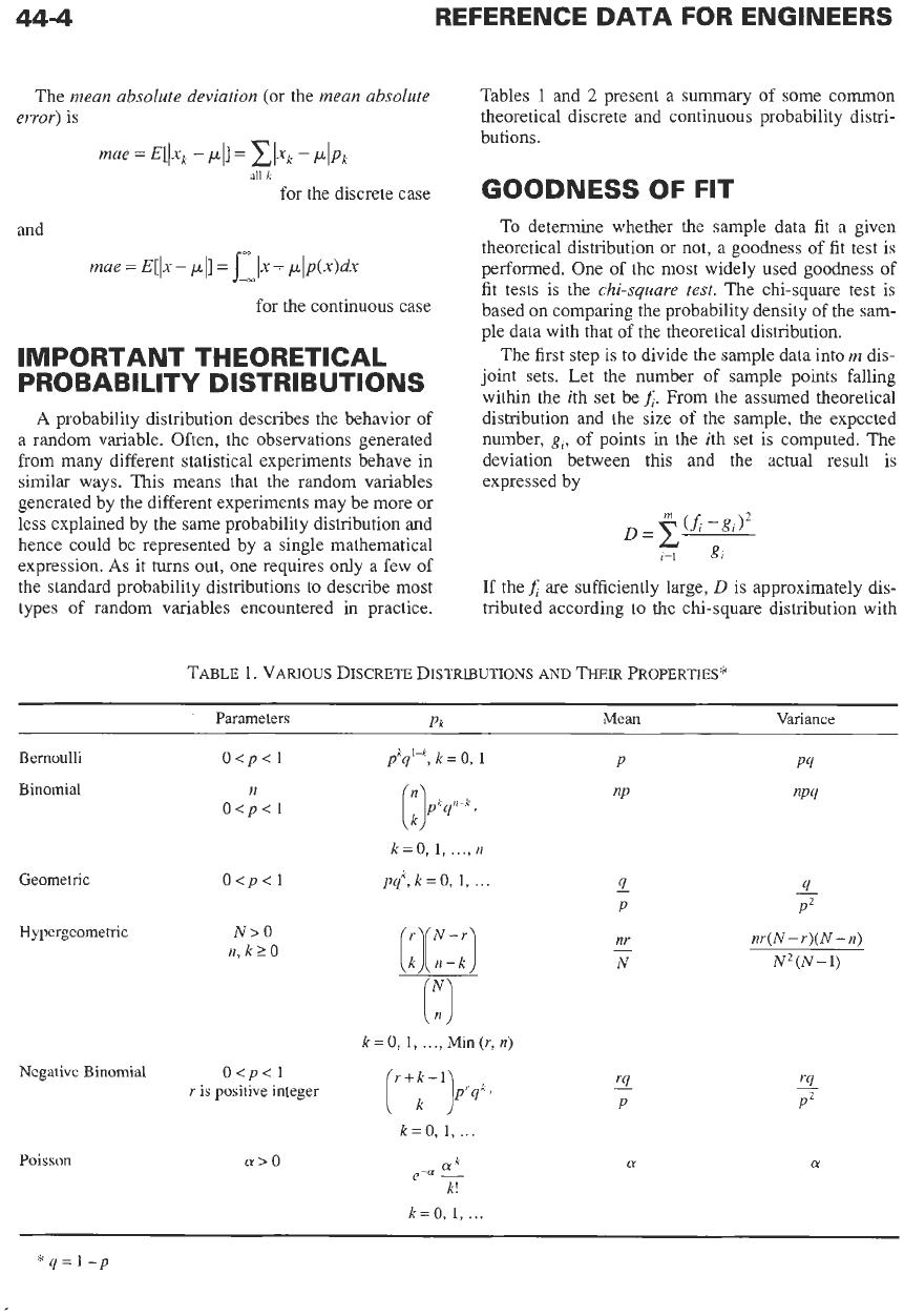
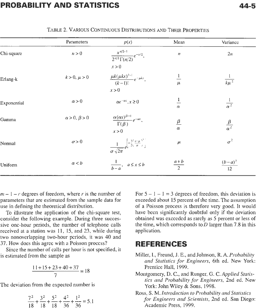
Tables
1
and
2
present a summary of some common
theoretical discrete and continuous probability distri-
butions.
GOODNESS OF FIT
To
determine whether
the
sample data fit a given
theoretical distribution or not, a goodness of fit test is
performed. One
of
the most widely used goodness of
fit tests is the
chi-square
test.
The chi-square test is
based
on
comparing the probability density of the sam-
ple data with that
of
the theoretical distribution.
The first step is to divide the sample data into
m
dis-
joint sets. Let the number
of
sample points falling
within the ith set be
A.
From the assumed theoretical
distribution and the size of the sample, the expected
number,
g,,
of points in the ith set is computed. The
deviation between this and the actual result
is
expressed by
If
theA are sufficiently large,
D
is approximately dis-
tributed according to the chi-square distribution with
TABLE
1.
VARIOUS
DISCRETE
DISTRI~UTIONS
AND
THEIR
PROPERTIES*
Parameters
Pk
Mean
Variance
Bernoulli
Binomial
Geometric
Hypergeometric
O<p<l
n
O<p<l
O<p<l
N>O
n,ktO
Negative Binomial
O<p<l
r
is
positive integer
pkq'-k,
k
=
0,
1
P
k=O,
1,
...,
n
pqh,k=O,
1,
...
13
k=
0,
1,
...,
Min
(r,
n)
4
P
-
nr
N
-
P4
nP4
4
-
P2
nr(N -r)(N
-
n)
N2(N
-1)
'4
-
P2
01
k=O,
1,
...
Poisson
01>0
a
k=O,
1,
..
*q=1-p
PROBABILITY AND STATISTICS
44-5
TABLE
2.
VARIOUS
CONTINUOUS
DISTRIBUTIONS
AND
THEIR
PROPERTIES
Parameters
P(X)
Mean
Variance
Chi-square
Erlang-k
Exponential
Gamma
Normal
Uniform
ff>O
a
>
0,
p
>
0
x>o
a>
0
[-i(Zg]
xe
a<b
1
a<x<b
b-a'
n
1
,u
-
1
-
a
P
-
a
,u
a+b
2
-
2n
(b
-
a)'
12
rn
-
1
-
r
degrees of freedom, where
r
11s
the number of
parameters that are estimated from the sample data for
use in defining the theoretical distribution.
To illustrate the application of the chi-square test,
consider the following example. During three succes-
sive one-hour periods, the number of telephone calls
received at a station was 11,
1.5,
and
2!3,
while during
two nonoverlapping two-hour periods, it was
40
and
37.
How does this agree with a Poisson process?
Since the number of calls per hour is, not specified, it
is estimated from the sample as
11
+
1.5
+
23
+
40
+37
7
=
L8
The deviation from the expected number is
72 32
52
42
12
-+-+-+-+-=5.1
18
18
18
36
36
For
5
-
1
-
1
=
3
degrees of freedom, this deviation is
exceeded about
1.5
percent of the time. The assumption
of a Poisson process is therefore very good. It would
have been significantly doubtful only if the deviation
obtained was exceeded as rarely as
5
percent or less
of
the time, which corresponds toD larger than
7.8
in this
application.
REFERENCES
Miller, I., Freund,
J.
E.,
and Johnson, R. A.
Probability
and Statistics for Engineers,
6th ed. New York
Prentice Hall, 1999.
Montgomery,
D.
C.,
and Runger,
G. C.
Applied Statis-
tics and Probability for Engineers,
2nd ed. New
York
John
Wiley
&
Sons,
1998.
for Engineers and Scientists,
2nd ed.
San
Diego:
Academic Press, 1999.
Ross,
S.
M.
Introduction to Probability and Statistics
45
Reliability
and
Life
-
Testing
Revised
by
Douglas
L.
Marriott
Definitions and Terminology 45-2
Reliability Definitions
45-5
Organization for Reliability
45-5
Elements of Reliability Assessment
45-6
Design Reviews
Failure Mode Analysis
Quantitative Reliability Assessment
Failure Data Collection and Assessment
Component Reliability
45-9
System Reliability
45-11
Sources of Reliability Data
45-13
Generic Data Sources
Life Testing
Probability and Statistical Inference
45-15
Confidence Limits
Fitting a Distribution Using Chi-Squared Test
Probability Paper
Weibull Analysis
Distribution-Free Tests of Goodness
of
Fit
Bayesian Statistics
Codes and Standards 45-25
The Use of Computers in Reliability
45-25
45-1