Massoud M. Engineering Thermofluids: Thermodynamics, Fluid Mechanics, and Heat Transfer
Подождите немного. Документ загружается.


762 VIc. Applications: Fundamentals of Turbomachines
The likelihood for cavitation increases with increasing specific speed conserva-
tively beyond about 8000.
Example VIc.3.7. The available NPSH for a pump delivering 50,000 GPM water
is 40 ft. Find the maximum impeller speed to avoid cavitation.
Solution: We find N from Equation VIc.3.2 with NPSH substituted for H
o
:
N = N
s
(NPSH)
3/4
/ V
1/2
:
N = 8000 × (40)
0.75
/(50,000)
1/2
= 569 RPM.
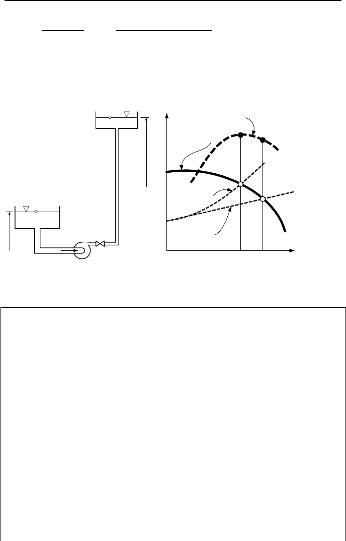
4. System and Pump Characteristic Curves
The challenge of selecting a pump is to meet the required capacity while providing
the required head at the point of best efficiency. Equation IIIb.4.8-1 (or IIIb.4.8-2)
gives serial-path system curves for laminar and turbulent flows. This is also plot-
ted in Figure VIc.4.1(b). Pump head and flow rate is obtained from the intersec-
tion of the pump characteristic and system curves. If this point does not corre-
spond with the point of peak efficiency, the pump speed should be adjusted
otherwise alternate pumps should be sought. We may try an analytical solution
for turbulent flow in pipes, for example where
2
31
VH
cc
System
+=
. Represent-
ing pump head versus flow rate with a parabola, we find H
Pump
= a + b
2
V
. Set-
ting the system head equal to the pump head, we find (b – c
3
)
2
V
+ (a – c
1
) = 0.
Flow rate is then found as
2/1
22
e
2/1
3
1
)]0H(V0)/V(H[)2/('
)(-0)V(H
V
¸
¸
¹
·
¨
¨
©
§
==+
−=
=
¸
¸
¹
·
¨
¨
©
§
−
−
=
¦
PumpPump
iPump
gDAfL
ZZ
bc
ca
VIc.4.1
where the two points to describe the H
Pump
= f( V
) are taken at maximum H and
maximum
V
. The flow rate calculated above should be checked against
o
V
,
flow rate corresponding to best efficiency point. If significant difference exists,
pump speed should be changed. If the change in speed still does not increase effi-
ciency, an alternate pump should be sought. To find if a change in speed brings
efficiency to its peak value, we use the homologous relations
'VV
CC = and C
H
=
C
H’
. If at N
o
rpm, the flow rate and head corresponding to peak efficiency are
o
V
and H
o
, then at any other speed these are given by )/(VV
oo
NN
= and H = H
o
(N/N
o
)
2
. We now substitute the new head and flow rate into the system curve to
get H
o
(N/N
o
)
2
= c
1
+ c
3
[]
2
oo
)/(V NN
. We solve this equation for N to get:
4. System and Pump Characteristic Curves 763
1/2
1e
oo
222
o3o o o
HV H['/(2)]V
i
CZZ
NN N
CfLgDA
¦
§· ½
−
°°
==
¨¸® ¾
−−
°°
©¹¯ ¿
VIc.4.2
Equation VIc.4.2 yields an acceptable answer only if the argument is greater than
zero. To increase accuracy, the pump curve should be represented by a higher or-
der polynomial.
i
e
Z
e
Z
i
Pump Head Curve
Pump Efficiency Curve
System Curve
Laminar FLow
System Curve
Turbulent
FLow
H
System
=
H
Pump
=
f
1
(V)
.
f
3
(V)
.
f
2
(V)
.
V
.
H
η
Pump
=
(a) (b)
Figure VIc.4.1. (a) Pump in a single-path system (b) Pump and system curves
Example VIc.4.1. The pump in Example VIc.3.1 is used to deliver water to a
height of 100 ft from the source reservoir. Total pipe length is 2000 ft and the
pipe diameter is 14 in. The pipe run includes a swing check valve, a fully open
gate valve, and a fully open globe valve as well as a total of 4 threaded 90° el-
bows. a) Find flow rate and efficiency. b) How do you maximize efficiency in
part (a)?
Solution: a) We first find the system curve from H
system
= c
1
+ c
3
2
V
where c
1
=
100 and c
3
is given by c
3
= fL’/(2gDA
2
).
However, L’ = L + L
e
. From Table III.6.3 (b), L
e
= 4 × 30 + 50 + 8 + 340 = 518
and from Table III.3.2, f = 0.013. Flow area becomes A =
π
(14/12)
2
/4 = 1.069 ft
2
.
Finally, c
3
= 0.013 × (2000 + 518)/[2 × 32.2 × (14/12) × 1.069
2
] = 0.38. There-
fore, H
system
= 100 + 0.38
2
V
, where flow rate is in ft
3
/s.
Approximating the pump head versus flow as a parabola (H
Pump
= a + b
2
V
), we
find coefficients a and b by using two points. The first point is at V
= 0, H
Pump
=
322 ft. Picking the second point at the best efficiency gives V
= 22000
GPM/(7.481 × 60) = 49 ft
3
/s and H
Pump
= 270 ft. This results in, a = 322 and b = –
0.0216 or H
Pump
= 322 – 0.0216
2
o
V
. From Equation VIc.4.1:
764 VIc. Applications: Fundamentals of Turbomachines
()( )
/sft51.23)38.00216.0/()322100(/a-cV
3
31
=−−−=−= cb
=
10552 GPM.
This corresponds to a head of 310 ft and an efficiency of about 73%, far from the
peak efficiency of 88%.
b) To increase the pump efficiency we may change the pump speed. To find the
new pump speed, we use homologous relations to get
o
V)710/('V
N= and H’ =
(N/710)
2
H
o
. We now substitute the new head and flow rate into the system curve
to get: (N/710)
2
× 270 = 100 + 0.38 {(N/710) [22000/(7.481 × 60)]}
2
. Thus, -
1.275E-3 N
2
= 100. It is clear we cannot reach peak efficiency for the operational
condition using this pump.
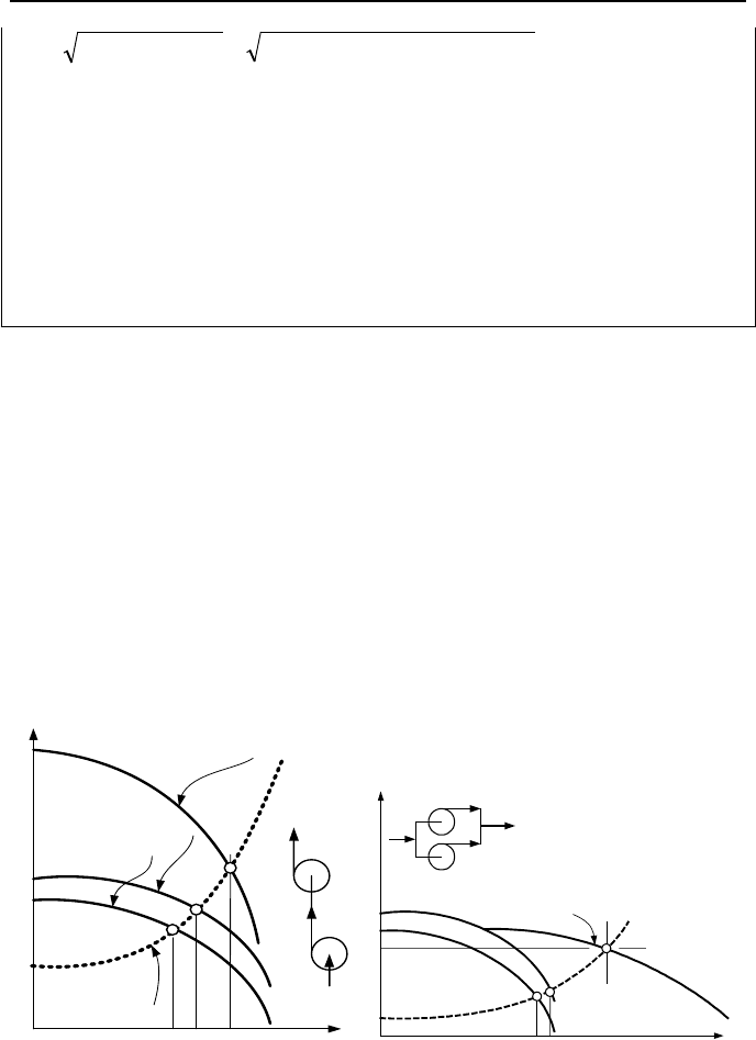
4.1. Compound Pumping System
Pumps may be used in serial or parallel arrangements depending on the flow or
head requirement. Pumps combined in series, as shown in Figure VIc.4.2(a) pro-
vide a higher head for the same flow rate and pumps combined in parallel, provide
the same head at higher flow rate. For optimum performance, not only the head
and flow rate of the compound pumping system must meet the demand but they
must also correspond to the point of best efficiency of each participating pump.
Compound pumping systems are not always used to meet the head and flow rate
demand. In many cases pumps are arranged in parallel to increase system avail-
ability.
V
.
H
H
P
u
m
p
A
+
P
u
m
p
B
=
f
1
(
V
)
+
.
f
2
(
V
)
.
H
System
=
f
3
(V)
.
H
Pump B
= f
2
(V)
.
H
Pump A
=
f
1
(V)
.
H
Pump A
=
V
.
H
H
Pump B
= f
2
(V)
.
H
System
=
f
3
(V)
.
f
1
(V)
.
V
B
.
V
A
.
V
.
=+
(a) (b)
Figure VIc.4.2. Compound pumping system in (a) serial and (b) parallel arrangements
4. System and Pump Characteristic Curves 765
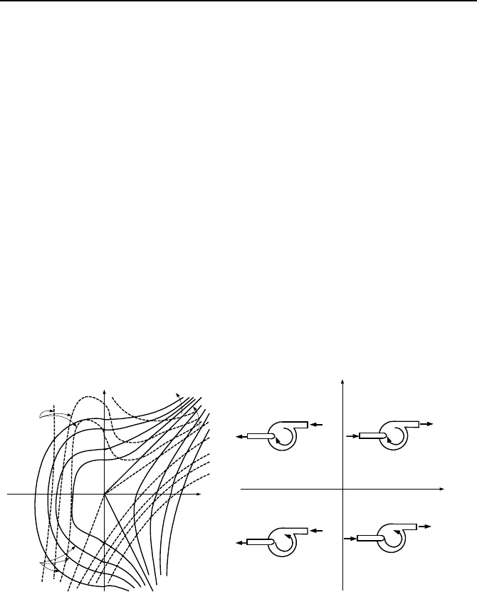
4.2. Extension of Pump Characteristic Curves
Earlier we discussed pump characteristic curves and the representation of the fam-
ily of such curves with the pump homologous curves. While it is desired that
pumps operate steadily at their rated condition, there are cases where pumps must
be analyzed for such off normal conditions as flow reversal in the pump and re-
verse rotation of the impeller. Such off normal operations require the extension of
the first-quadrant pump characteristic curves (positive flow rate and positive
speed) to all four quadrants where any combination of positive and negative flow
rate and speed exists. Unlike Figure VIc.3.1, where head and volumetric flow rate
are chosen as coordinates, as shown in Figure VIc.4.3(a), the coordinates are cho-
sen to be volumetric flow rate and the impeller speed. The resulting plots, as em-
pirically produced by the pump manufacturer, are known as the synoptic curves,
which constitute the Karman-Knapp circle diagram. In this figure, the solid lines
represent constant head and the dotted lines show the constant pump hydraulic
torque. Figure VIc.4.3(b) shows possible modes of operation of a pump during a
transient. The first quadrant is normal pump (N). The solid lines between H = 0
and the speed coordinate are the familiar head versus flow rate curves. Expect-
edly, for a constant flow rate, head increases with increasing impeller speed.
There are also lines representing negative pump head in this quadrant for positive
flow and positive impeller speed.
V
.
N
C
o
n
s
t
a
n
t
T
o
r
q
u
e
C
o
n
s
t
a
n
t
H
e
a
d
-
1
0
0
%
0
%
5
0
%
1
0
0
%
-
5
0
%
0%
0
%
5
0
%
100%
-
2
5
%
-
5
0
%
-
1
0
0
%
Q
.
N
Normal
Pump
Energy
Dissipation
Reverse
Pump
Normal
Turbine
HAN HVN
BAN BVN
HAD HVD
BAD BVD
HAT HVT
BAT BVT
HAR HVR
BAR BVR
N
D
T
R
(a) (b)
Figure VIc.4.3. (a) Pump characteristic curves in four quadrants and (b) Possible modes of
operation
In the second quadrant (D), we find only positive pump head for positive im-
peller speed but negative flow rate. The third quadrant (T) is referred to as normal
turbine where, for positive pump head, flow direction is into the pump with the
impeller rotating in the reverse direction. Finally, in the forth quadrant (R) there
are both positive and negative pump heads for positive flow and reverse impeller
rotation. It is obvious that representation of such massive pump characteristic data
766 VIc. Applications: Fundamentals of Turbomachines
in computer analysis is impractical. Therefore, we resort to the non-dimensional
homologous curves to represent the pump characteristic curves. This, in turn, re-
quires the definition of some additional non-dimensional groups.
For a given pump, we use the rated data, which correspond to the point of best
efficiency, to normalize variables. Hence, we obtain speed ratio (a =
ω/ω
o
=
N/N
o
), flow ratio (v =
o
V/V
), head ratio (h = H/H
o
) and torque ratio (b = T/T
o
).
The flow, head, and torque coefficients now take the form of
V
C = b/v, C
H
= h/a
2
,
and C
T
= b/a
2
, respectively. We then can find C
H
and C
T
as functions of
V
C .
During analysis of pump response to a transient flow rate and impeller speed trav-
erse positive and negative values. As such, both variables may encounter zero. In
the case of the impeller speed, the values of the above coefficients would be unde-
termined. To avoid such conditions, we update our definition of the above coeffi-
cients and produce
2'
H
h/b=C and
2'
v/b=
T
C .
Generally, the head or torque coefficients (C
H
and C
T
or
'
H
C and
'
T
C ) as inde-
pendent variables are expressed in terms of flow and speed ratios (a and v). Since
there are also four quadrants where these independent variables should be deter-
mined, it has become customary to use shorthand (a three-letter notation) to iden-
tify various variables in various quadrants. The first letter identifies the dependent
variables (i.e., whether we are dealing with head or torque (h or b)). Hence, H
designates head and T designates torque ratios. The second letter, as a representa-
tive of the independent variable, is such that A designates division by a for the in-
dependent variable, and division by a
2
for the dependent variable. Similarly, V
designates division by v for the independent variable and division by v
2
for the
dependent variable. Finally, the third letter indicates the mode in which the pump
is operating, as shown in Figure VIc.4.3(b). These modes are N, R, T, and D for
Normal pump, Reverse pump, normal Turbine, and energy Dissipation, respec-
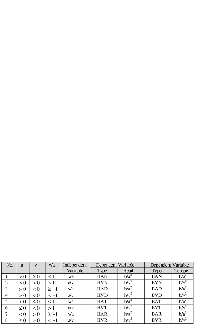
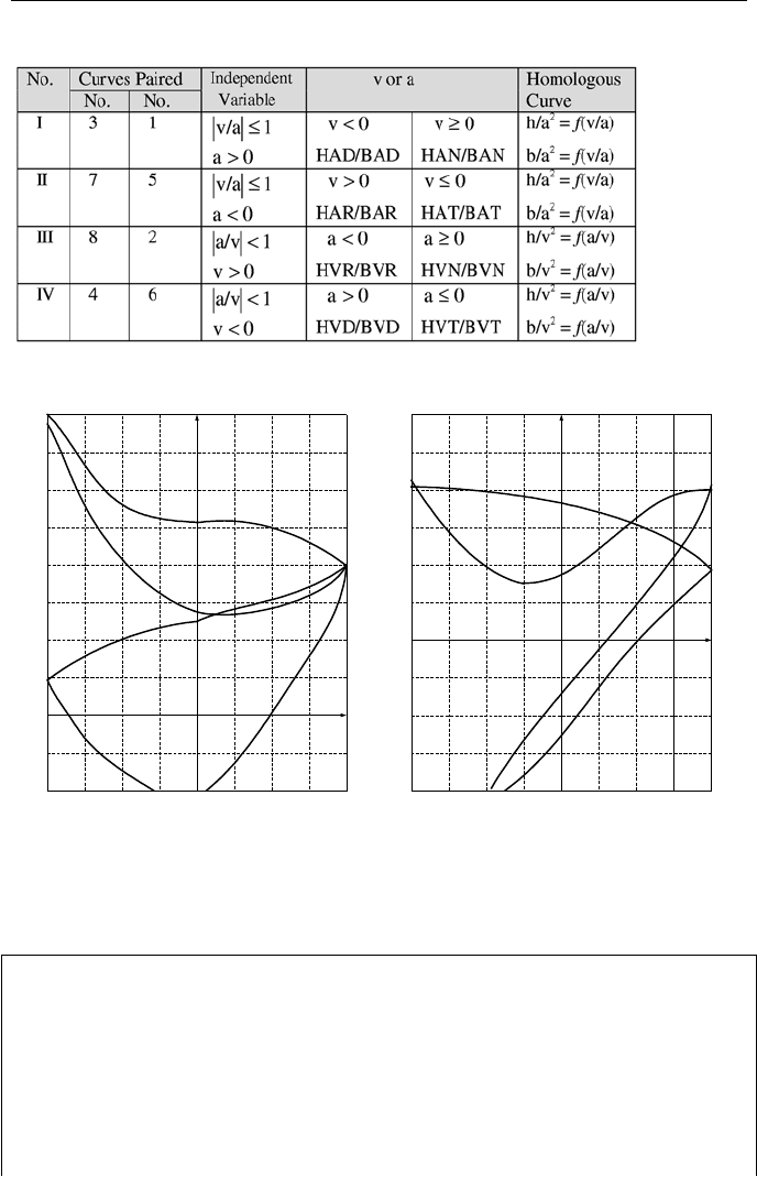
tively. These conventions are summarized in Table VIc.4.1, which defines 16
curves: 8 for head and 8 for torque. We now group similar curves of Ta-
ble VIc.4.1 to obtain only four curves as summarized in Table VIc.4.2. These four
homologous curves are shown for a typical centrifugal pump in Figure VIc.4.4(a)
for homologous head and in Figure VIc.4.4(b) for homologous torque.
Table VIc.4.1. Summary of homologous curve notations
4. System and Pump Characteristic Curves 767
Table VIc.4.2. Determination of pump homologous curves from pump characteristic curves
2.0
1.5
1.0
0.5
0.0
-0.5
-1.0
-0.5
0
0.5
1.0
HAD
HAN
HVD
HVT
HAT
HAR
HVR
HVN
h/v
2
h/a
2
or
v/a or a/v
1.5
1.0
0.5
0.0
-0.5
-1.0
-1.0
-0.5 0
0.5 1.0
BVD
BAN
BAD
BVT
BVN
BAT
BVR
BAR
b/v
2
b/a
2
or
v/a or
a/v
(a) (b)
Figure VIc.4.4. Dimensionless homologous (a) pump head and (b) hydraulic torque
Example VIc.4.2. In a transient, the speed and flow rate of a centrifugal pump
are given as N = –600 rpm and V
= –200,000 GPM. Find a) pump head and
torque, b) pump efficiency, and c) the temperature rise of the liquid across the
pump for rated conditions. The rated values of the pump are:
N
o
= 900 rpm,
o
V
= 370,000 GPM, H
o
= 270 ft, T
o
= 136,000 ft·lbf, and
ρ
= 50 lbm/ft
3
.
Solution: a) Having V
and N, we obtain v = V
/
o
V
= –200,000/370,000 = –
0.54 and a = N/N
o
= –600/900 = –0.67. Hence, a/v = –0.54/–0.67 = 0.81.
768 VIc. Applications: Fundamentals of Turbomachines
From Figure VIc.4.4(a), using the HVT curve we find for a/v = 0.81, h/v
2
= c
1
≅
0.8
From Figure VIc.4.4(b), using the BVT curve we find for a/v = 0.81, b/v
2
= c
2
≅
0.6. Therefore,
H = hH
o
= 0.8 × (0.54)
2
× 270 = 63 ft and T = bT
o
= 0.6 × (0.54)
2
× 136,000 =
24,588 ft·lbf.
b) It can be easily shown that pump efficiency is related to the rated efficiency as
η
/
η
o
= (c
1
/c
2
)(v/a)
Having c
1
and c
2
from (a), and
η
o
, we can find
η
. However, pump efficiency is
defined for the first quadrant. In the third quadrant for example, where the pump
is in the turbine mode, efficiency should be redefined to fit the mode of operation.
c) Total power delivered to the liquid is
BHP
W
=
ρ
o
g
o
V
H
o
. This is equal to the
energy gained by the water as given by Tc
po
∆
o
V
ρ
. Hence, ∆T = H
o
g/c
p
. If the
liquid is water, c
p
= 1 Btu/lbm F = 778 ft·lbf/lbm F. Hence, ∆T = 270/778 =
0.35 F.
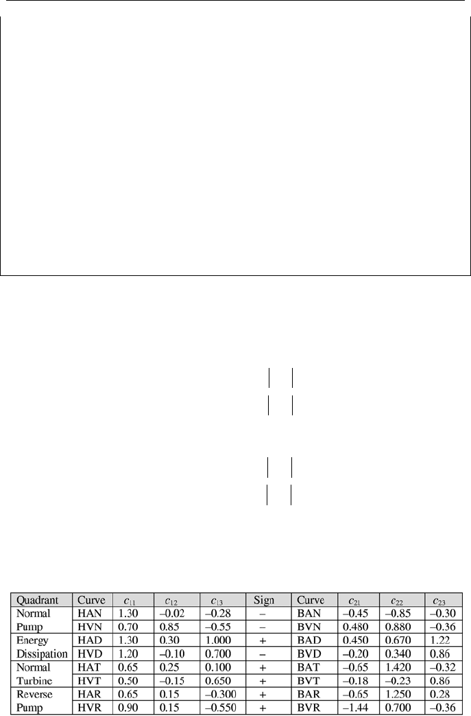
Since production of the pump homologous curves is tedious, there are several
attempts to represent these by polynomial curve fits. For example, Streeter rec-
ommends parabolic functions for the representation of these curves in various
quadrants. The dimensionless head becomes:
2
131211
)a(v/(v/a)h ccc ++= 1v/a0 ≤≤ VIc.4.1-1
2
111213
)a/v((a/v)h ccc ++= 1v/a > VIc.4.1-2
and the dimensionless hydraulic torque:
2
232221
/v)a((a/v)b ccc ++= 1v/a0 ≤≤ VIc.4.2-1
2
232221
/v)a((a/v)b ccc ++= 1v/a > VIc.4.2-2
using the coefficients c
ij
given in Table VIc.4.3.
Table VIc.4.3. Coefficient for parabolic fit to pump homologous curves

5. Analysis of Hydraulic Turbines 769
Having the curve fit coefficients and the rated values, flow rate and hydraulic
torque are found from:
()
[]
{
}
2/1
131311
2
121213o
h4a4signa)2/V(V cccccc +−+−=
()
2
2322
2
21oH
vavaTT ccc ++=
Another example for curve fitting to the pump homologous curve is given by Kao
as polynomials:
¦
=
−
=
4
1
1
3
2
)v/a(h/a
i
i
i
c and
¦
=
−
=
4
1
1
4
2
)v/a(b/a
i
i
i
c
where coefficients c
31
through c
34
for positive impeller speed are 1.80, –0.30, 0.35
and –0.85 and for negative impeller speed are 0.50, 0.51, –0.26, 0.25. For dimen-
sionless torque, coefficients c
41
through c
44
for positive impeller speed are 1.37, –
1.28, 1.61, and –0.70 and for negative impeller speed are –0.65, 1.9, –1.28,
and 0.54. In a transient, if the impeller speed goes to zero when changing direc-
tion from positive to negative speed, the pump head versus flow for these sets of
polynomial curves may be found from:
vv)3181.4(h −−= E
While theoretically a centrifugal pump may operate in all four quadrants, in prac-
tice, pump operation in the first quadrant can be ensured by pump and system
modification. For example, installing a non-reversing ratchet prevents the impel-
ler from rotating in the reverse direction and a check valve on the discharge line
prevents reverse flow into the pump.
5. Analysis of Hydraulic Turbines
Turbines are mechanical devices to convert the energy of a fluid to mechanical
energy. Turbines can be classified in various ways based on process, head con-
version, or rotor type. Regarding the process, energy transfer in turbines may take
place in either an adiabatic or in an isothermal process. Regarding head conver-
sion, turbines may be divided into the reaction and the impulse type for momen-
tum exchange between fluid and the turbine rotor. Finally, turbines may be classi-
fied depending on the velocity vector resulting in an axial, radial, or mixed-flow
rotor.
5.1. Definition of Terms for Turbines
Adiabatic process turbines, as were studied in Chapter IIb, include gas and
steam turbines where the means of energy transfer from fluid to the turbine rotor is
primarily through the change in the fluid enthalpy. In this type of turbine, changes

770 VIc. Applications: Fundamentals of Turbomachines
in the fluid potential and kinetic energy are generally negligible, compared with
the change in fluid enthalpy.
Isothermal process turbines include turbines used in greenpower production
such as hydropower and wind turbines. In this type of turbine, the transfer of me-
chanical energy to the turbine rotor is due to the fluid kinetic energy, while
changes in enthalpy are generally negligible compared with the change in the fluid
kinetic energy.
Reaction type turbines or simply reaction turbines, have rotors equipped with
blades. In the reaction type turbines, fluid fills the blade passages of the rotor to
deliver momentum. Thus, the head conversion in the reaction type turbines occurs
within the turbine rotor where fluid pressure changes from inlet to outlet. Exam-
ples of the reaction type turbines include adiabatic, wind, and most hydropower
turbines.
Impulse type turbines convert the head in an injector. Thus, in an impulse
turbine, the head conversion takes place outside the turbine rotor. The high veloc-
ity jet then strikes individual buckets attached to the Pelton wheel at a constant
pressure. Imparting the momentum of the jet to a bucket produces a force, which
results in a torque to turn the wheel and brings the adjacent bucket to face the jet.
5.2. Specific Speed for Turbines
The same dimensionless groups defined in Section 3 for pumps are also applicable
to turbines. Recall that for pumps we expressed the head and the power coeffi-
cient in terms of the capacity coefficient. However, for turbines, we express the
capacity and the head coefficient in terms of the power coefficient. In the U.S., it
is customary to find specific speed for turbines from:
4/5
2/1
)ftH,(
)bhp)(rpm,(N
N
s
=
VIc.5.1
5.3. Adiabatic Turbines, Steam Turbine
The adiabatic turbines, regardless of the type of working fluid, are generally of ax-
ial flow type. However, turbines used for turbo-charging are generally of radial
flow type.
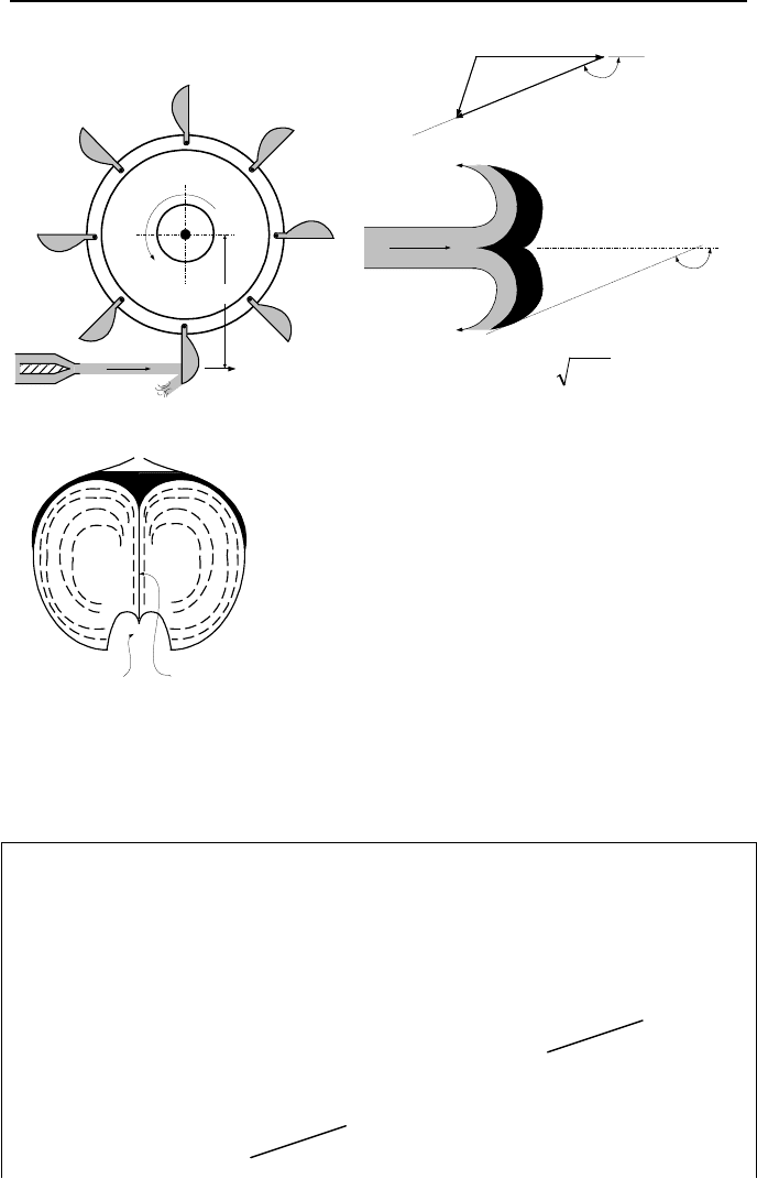
5.4. Isothermal Turbines, Pelton Turbine
As discussed in Chapter I, Pelton wheels are impulse turbines in which high head
and low flow rate of water strikes the buckets attached to the wheel, as shown in
Figure VIc.5.1. Our goal is to determine the Pelton wheel in terms of the jet ve-
locity (V
j
), the bucket velocity (V
t
), and the bucket angle (
β
). This is shown in the
example that follows.
5. Analysis of Hydraulic Turbines 771
R
V
t
= 2
π
NRV
j
N, ω
V
j
β
≈
165
o
V
j
V
t
V
β
≈ 165
o
α
H2gCV
vj
=
(a) (b)
SpearSlit
Split-cup Bucket
(c)
Figure VIc.5.1. Pelton wheel. (a) Side view of the wheel, (b) & (c) top and frontal views
of the bucket.
Example VIc.5.1. Derive the efficiency of the Pelton wheel in terms of the con-
stant velocities V
j
, V
t
, and the jet reflection angle of
β
.
Solution: Efficiency of the wheel is defined as the ratio of the power obtained
from the wheel to the power delivered to the wheel
inout
WW
/=
η
(i.e., the break
horsepower to the hydraulic horsepower).
()
()( )
()
[
]
2/V//2/1/2//
2222
jjjjjin
VdtdVmVdtdmdtmVddtdEW
ρ
=+===
We find
out
W
from the rate of change of momentum for which we must consider
the relative velocities.
F = d(mV)/dt = (dm/dt)V + (dV/dt)m = V
V
ρ
. Note that V = V
j
– V
t
. The net force
applied on the wheel is