Luo A.C.J. (Ed.) Dynamical Systems: Discontinuity, Stochasticity and Time-Delay
Подождите немного. Документ загружается.


27 Inversely Found Elastic and Dimensional Properties 343
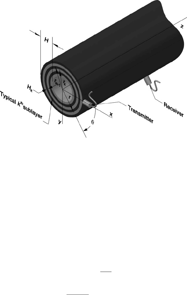
Fig. 27.1 A pipe’s discretization
to be uniformly right circular, homogeneous, linearly elastic and isotropic. It has
Lam´e constants and , density , a constant mean radius R, outside radius r
0
and thickness H , in addition to traction free, inner and outer surfaces. Right hand
cylindrical and Cartesian coordinate systems .r; ; z/ and .x; y; z/, respectively, are
shown in Fig. 27.1. Their common origin is located at the geometric centre of a
generic cross-section of the pipe with the z axis directed along the pipe’s longitudi-
nal (axial) axis.
The point excitation, F
t
.; z;t/, is applied normally to the external surface at
y D 0 in the plane z D 0 by the transmitting transducer. (In the cylindrical
coordinate system, the excitation’s application coincides with D 0.) To circum-
vent convergence difficulties associated with a point application, the excitation is
approximated by using a “narrow” pulse having a uniform amplitude over a circum-
ferential distance 2r
0
0
. This narrow pulse is represented by using a Fourier series of
“ring-like” loads having separable spatial and time, t, variations. In particular,
F
t
.; z;t/ D F
0
p.t/•./•.z/
(
p.t/
2r
0
0
•.z/F
0
;
0
0
0; otherwise
D
1
X
nD1
sinc.n
0
/
2r
0
e
jn
•.z/F
0
p.t/; (27.1)

344 D.K. Stoyko et al.
where use has been made of the Fourier series for a rectangular pulse. In (27.1) F
0
and p.t/ are a vector and a function that describe the radial and temporal variations
of the excitation, respectively, n is the circumferential wave-number, ı is the Dirac
delta function, and j D
p
1.TheF
0
is a vector of zeros except for a single element
corresponding to the excitation’s specified position and direction. Application of
the Fourier transform integral to the series in (27.1) transforms the excitation vector
from the axial, z, domain to the wave-number, k, domain. The result is:
F
t
.;k;t/
1
X
nD1
sinc.n
0
/
2r
0
e
jn
F
0
p.t/; (27.2)
in which the “sifting” property of the Dirac delta function has been applied.
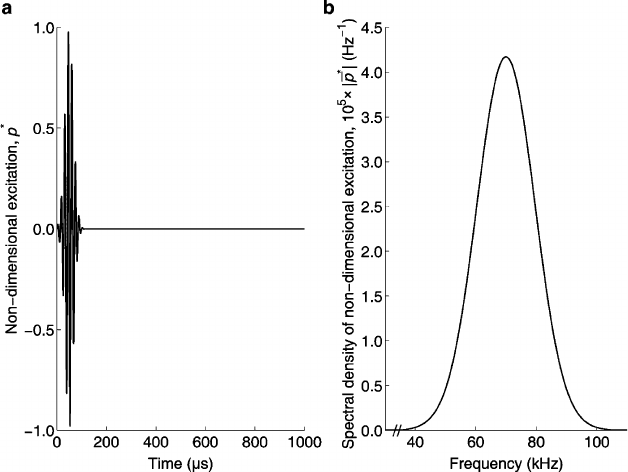
In (27.1)and(27.2) p.t/ is taken as the commonly used Gaussian modulated sine
wave, which has a non-dimensional form (always indicated by a star superscript) of
p
.t/ D
H
p.t/ D
(
0; t < 0
e
a.ht/
2
sin.h!
0
t/; t 0:
(27.3)
The constant a, , !
0
,andh are:
a D 2:29595 10
10
s
2
; (27.4a)
D 1:4 10
5
s; (27.4b)
!
0
D .5 10
5
/ rad=s; and (27.4c)
h D 0:28 (27.4d)
here. Consequently the excitation has a 70 kHz centre frequency and over 99%
of its energy is contained within a 35–107kHz bandwidth. Therefore, the Fourier
integral transform of p
.t/, Np
.!/ where ! is the circular frequency, may be rea-
sonably assumed to be contained within this finite bandwidth. The adopted p
.t/
and
j
Np
.!/
j
, where an over bar indicates a Fourier transformed variable, are illus-
trated in Fig. 27.2.
Having described the excitation, its effect on the pipe has to be considered next.
The pipe is discretized into N layers through its thickness, where N is six in
Fig. 27.1. The thickness of the kth layer is H
k
, and it extends radially from r
k
to r
kC1
. For simplicity, the H
k
are considered to be identical. Each layer corre-
sponds to a one-dimensional finite element in the pipe’s radial direction for which a
quadratic interpolation function is assumed. A conventional finite element approach
is applied, layer by layer, to approximate the elastic equations of motion [21]in
which the displacements, u
t
.r; ; z;t/, take the form
u
t
.r; ; z;t/ D N.r/U
t
.; z;t/: (27.5)
The N.r/ contains the set of interpolation functions assembled over the entire
pipe. On the other hand, U
t
.; z;t/ assimilates the corresponding array of nodal

27 Inversely Found Elastic and Dimensional Properties 345
Fig. 27.2 Applied excitation in (a) time and (b) frequency
displacements in which the easily measured radial displacement at the pipe’s ex-
ternal surface is principally of interest. Like the similarly approximated excitation
F
t
.; z;t/,theU
t
.; z;t/is assumed to be circumferentially periodic, i.e.,
U
t
.; z;t/ D
1
X
nD1
e
jn
U
t
n
.z;t/: (27.6)
Consider, on the other hand, a single temporally harmonic component of
F
t
.; z;t/, F.; z;t/, having (circular) frequency !. This excitation component
produces the harmonic response component U.; z;t/. The Fourier series of these
two variables take the form:
U.; z;t/ D e
j!t
1
P
nD1
e
jn
U
n
.z/
(27.7a)
and
F.; z;t/ D e
j!t
1
P
nD1
e
jn
F
n
.z/:
(27.7b)
Equations (27.7a)and(27.7b) are substituted into approximate equations of
motion obtained from Hamilton’s principle [21]. The result is transformed into the
346 D.K. Stoyko et al.
wave-number domain by applying the Fourier integral transform and making use of
(27.2). The result for the nth circumferential wave-number is:
K
1
C jnK
2
C n
2
K
4
!
2
M
N
U
n
C jnk
n
.K
3
jnK
5
/
N
U
n
Ck
2
n
K
6
N
U
n
D
N
F
n
; (27.8)
where the K
i
are stiffness matrices and M is the mass matrix. Details are given
in [21].
Proceeding in a classical modal analysis fashion, (27.8) takes the form of an
eigensystem in the special case when
N
F
n
is the null vector. Integer values are always
assigned to n. Either k
n
or ! is assigned when the wave-number or frequency is
presumed. Then a linear or quadratic eigensystem is produced in !
2
or k
n
, respec-
tively. In the latter, more commonly encountered case, (27.8) may be rewritten in
the linear form:
ŒA.n; !/ k
n
B
N
U
n
k
n
N
U
n
D
0
N
F
n
; (27.9)
where:
A.n; !/ D
0I
K
1
C jnK
2
C n
2
K
4
!
2
M
jn.K
3
jnK
5
/
; (27.10a)
B D
I0
0 K
6
(27.10b)
and 0 (I) is the null (identity) matrix.
Normal modes are found for the nth circumferential wave-number by solving
the homogeneous form of (27.9). This results in 12N C 6 eigenvalues or axial
wave-numbers. A real (complex) valued wave-number corresponds to a propagat-
ing (evanescent) wave. Moreover, half the wave-numbers correspond to solutions
for the positive z coordinates; the other half represent solutions for the negative z
coordinates. In addition to the wave-numbers, right and left eigenvectors,
R
nm
and
L
nm
respectively, are associated with the mth eigenvalue. They are partitioned into
the upper and lower halves.
R
nm
D
˚
R
nmu
R
nml
T
(27.11a)
and
L
nm
D
˚
L
nmu
L
nml
T
(27.11b)
that are represented by the subscripts u and l, respectively.
The pipe’s response is obtained, for the nth circumferential wave-number and
only those axial cross sections having positive z, by linearly superimposing the ad-
missible 6N C3 right eigenvector solutions. Applying first the inverse Fourier trans-
form to this sum, and then Cauchy’s residue theorem, gives the nth circumferential
mode of the response. The result is [21]:

27 Inversely Found Elastic and Dimensional Properties 347
U
n
.; z;t/ De
j!t
jsinc.n
0
/
2r
0
6N C3
X
mD1
L
nml
T
F
0
B
nm
R
nmu
e
jk
nm
z
; (27.12)
where
B
nm
•
mp
D
L
nm
T
B
R
np
; (27.13)
in which bi-orthogonality relations [20] have been used. Moreover, •
mp
is the
Kronecker delta. The linear response to a multi-frequency excitation can be found
by merely superimposing the responses caused by each individual frequency com-
ponent. Hence:
U
t
.; z;t/ D
j
4
2
r
0
Z
1
1
Np.!/e
j!t
1
X
nD1
sinc.n
0
/
"
6N C3
X
mD1
L
nml
T
.!/F
0
B
nm
.!/
R
nmu
.!/e
jk
nm
.!/z
#
e
jn
d!
(27.14)
after summing all the circumferential harmonic components.
27.3 Simplifying Features
It is demonstrated in [17,18], by using the modal decomposition capability of SAFE,
that the “peak” magnitudes of a pipe’s radial F
requency Response Function (FRF)
occur at its modal cut-off frequencies where the wave number is zero. A sharp
increase there arises because the corresponding B
nm
in (27.12)and(27.13) tends
to zero as a cut-off frequency is approached, i.e., a singularity happens in the
nm mode’s FRF. Although details are omitted here for brevity, this feature ex-
ists because there is a repeated root at each cut-off frequency. Hence a defective
1
eigensystem exists. Consequently the corresponding left and right eigenvectors are
orthogonal to the B matrix defined in (27.10)andB
nm
also becomes zero [20]. It
is interesting that a cut-off frequency can be interpreted as a juncture at which a
travelling wave problem transitions to a vibration problem because the wavelength,
2=k
nm
, becomes infinitely long. Therefore, the response at a cut-off frequency may
be termed “vibration”-like [6,12]. Also note from (27.14) that a modal response at
a cut-off frequency becomes advantageously independent of an observation point’s
axial location. Moreover, cut-off frequencies can be calculated without knowing the
corresponding eigenvectors of (27.8) with k
n
D 0 and
N
F
n
D 0.
Cut-off frequencies depend, through the stiffness and mass matrices, on the
pipe’s elastic properties, mass density, and geometrical dimensions. It is assumed
1
A defective eigensystem is one in which an eigenvalue is repeated, say integer r times, but fewer
than r unique (right) eigenvectors exist for the repeated eigenvalue [20].

348 D.K. Stoyko et al.
here that the pipe’s outer diameter and mass density are readily available, which
leaves the elastic properties and wall thickness to be determined. Two independent
elastic constants are sufficient to characterize a homogeneous isotropic material.
The Buckingham theorem [5] is used to reduce the dimensional space and make
calculations more tractable. Then, for a given circumferential wave-number n and
order m, the non-dimensional cut-off frequency ratio
!
c
F.n;m/
D
!
c
F.n;m/
!
ref
(27.15)
is defined where !
ref
D 1=H
p
.=/ and !
c
F.n;m/
is the cut-off frequency of
the F.n; m/ flexural mode.
2
The !
c
F.n;m/
can be expressed in terms of the non-
dimensional parameters .H=R/ and .=/. Note that the desired elastic properties
and wall thickness can be calculated from .H=R/, .=/,and!
ref
,aswellasthe
presumed mass density and outer diameter [18,19]. The inequality 0<.H=R/<2
arises physically because the lower and upper bounds relate to a pipe having no wall
thickness and a solid pipe, respectively. On the other hand, .=/ can be bounded
reasonably as 0 .=/ . 10 from the standard elasticity relation 0 0:5,
where is Poisson’s ratio.
27.4 Graphical Relations Between the Cut-Off Frequencies
and Cylinder Properties
The key to making the inverse problem tractable is a succinct yet clear presenta-
tion showing the dependence of the forward solved cut-off frequencies upon the
independent !
ref
, .H=R/ and .=/. Transformations to obtain practical engineer-
ing properties, which also require the use of f D !=.2/ where f is frequency,
are performed later. The presentation’s construction may be envisaged by initially
considering all the , H , ,and!
ref
to be unity. Then and R are each varied uni-
formly within the physically viable ranges described earlier. Forward computations
to determine three non-dimensional cut-off frequencies, say !
c
F.10;1/
, !
c
F.11;1/
and
!
c
F.12;1/
, are performed within these ranges by SAFE. The corresponding values of
.H=R/ and .=/,given!
ref
is simply 1 rad=s, are also noted.
In general
!
c
F.i;1/
D
!
c
F.i;1/
!
ref
for all i; (27.16)
so that a particular !
c
F.i;1/
is identical to !
c
F.i;1/
at this juncture. Moreover
!
c
F.10;1/
!
c
F.11;1/
!
c
F.12;1/
(27.17)
2
Modes are labelled by using the standard convention employed in [16]. Only flexural modes are
considered here although the extension to torsional or longitudinal modes is obvious.

27 Inversely Found Elastic and Dimensional Properties 349
regardless of the value of !
ref
. Then the largest of the three !
c
F.i;1/
, !
c
F.12;1/
,is
taken as an extreme but arbitrary 200;000 rad=s(i.e.,f
c
F.12;1/
is 100 kHz). The
non-dimensional cut-off frequency for the selected values of .H=R/ and .=/ are
available so that equation (27.16) is used to find the corresponding !
ref
.Theas-
sociated values of !
c
F.10;1/
and !
c
F.11;1/
can be determined similarly. Two points
!
c
F.10;1/
;!
c
F.11;1/
;!
c
F.12;1/
, computed for the assumed (unity) and calculated !
ref
,
are converted to frequencies, in kHz, and graphed. They are joined by a line along
which .H=R/ and .=/ are each constant, but !
ref
varies. The line must also pass
through the graph’s origin because, physically, the !
c
F.i;1/
and !
ref
are zero there.
The effects of other variations in !
ref
are calculated straightforwardly. The same
procedure produces a set of similar, closely spaced lines after perturbing .H=R/
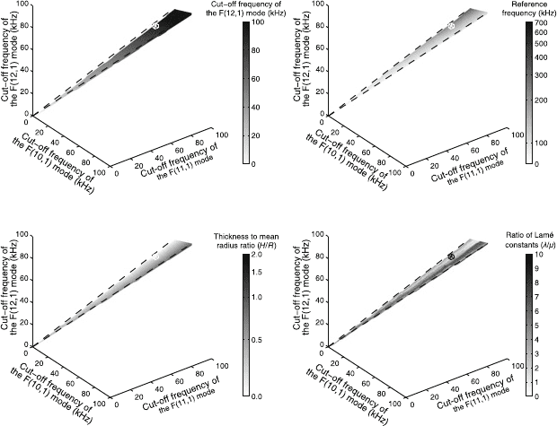
and .=/. The resulting overall behaviour is presented in Fig. 27.3.
The shaded solution space of Fig. 27.3a shows the dependence of !
c
F.12;1/
(or, al-
ternatively f
c
F.12;1/
) upon !
c
F.10;1/
(f
c
F.10;1/
)and!
c
F.11;1/
(f
c
F.11;1/
). Note that three
cut-off frequencies are required to determine the three unknown .H=R/, .=/ and
!
ref
. The solution space seems to be a narrow bounded plane whose width increases
progressively with deepening shades, i.e., higher f
c
F.12;1/
. This is somewhat decep-
tive, however, because a computed inverse solution has been found empirically to
ab
cd
Fig. 27.3 Dependence of the three cut-off frequencies on (a) each other, (b) f
ref
D !
ref
=2,
(c) .H=R/,and(d) .=/. A dashed line indicates a boundary

350 D.K. Stoyko et al.
exist only in a thin volume, not on a planar approximation. Previous research [18,19]
supports this contention because it was determined that cut-off frequencies should
be measured ideally within 0.01%.
The shadings of Figs. 27.3band27.3c indicate that the cut-off frequencies de-
pend strongly upon f
ref
or !
ref
and .H=R/, particularly at their highest values.
Interestingly, a quite uniform shading emerges when these two figures are superim-
posed. Therefore, similar changes in f
ref
and .H=R/ counterbalance. On the other
hand, the sizeable swathes of a given shading seen in Fig. 27.3d suggest that the
f
c
F.i;1/
, i D 10; 11; 12, alter little with large .=/ modifications. A comparison
of Fig. 27.3c, d also intimates that shadings across the shorter width of the solu-
tion space have similar tendencies for the .=/ and smaller .H=R/ variations.
Therefore, the effect of .=/ may be concealed, to some extent, by a greater one
from .H=R/.
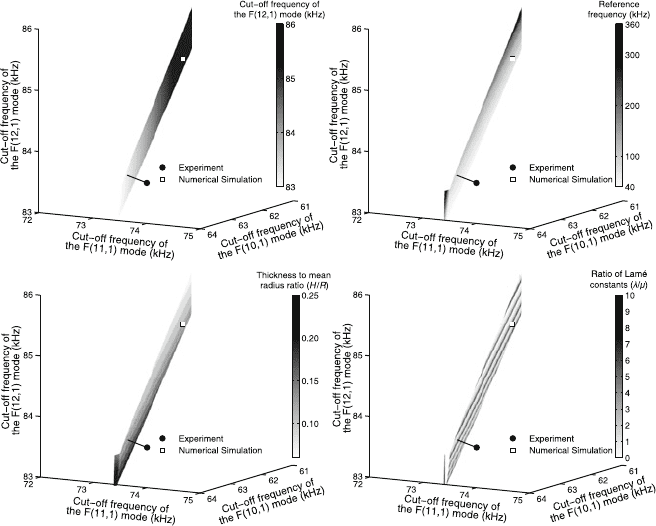
Figure 27.4 is a magnification of the computed solution space and nearby regions
contained within the boxes shown in Fig. 27.3. The illustrated points, which are off-
set slightly from the surface, correspond to the cut-off frequencies extracted from
simulated and experimentally measured time histories, to be presented later. The
off-sets arise from uncertainties and errors, the overall magnitudes of which are
ab
cd
Fig. 27.4 Magnified version of Fig. 27.3 near the experimental and simulated data; dependence of
the three cut-off frequencies on (a) each other, (b) f
ref
D !
ref
=2,(c)(H/R), and (d)(=)

27 Inversely Found Elastic and Dimensional Properties 351
intimated by the off-set’s shortest distance to the computed surface. The errors arise
principally from the temporal curve fitting procedure to find the cut-off frequencies.
Numerical studies [19] suggest that all the discernible cut-off frequencies in the
measurement bandwidth should be incorporated to reduce the error. Uncertainties,
on the other hand, may originate from any questionable assumption of SAFE like
complete uniformity, no out-of-roundness, homogeneity, etc.
27.5 Inversion Scheme
The transmitter is pulsed using the previously described excitation and the response
is measured by the nearby receiving transducer. Three cut-off frequencies, O!
c
F.n
i
;m
i
/
,
are “extracted” from the measured transient response using the temporal curve fit-
ting procedure described in [19]. If these cut-off frequencies are exact and the SAFE
modelling is perfect, the following relations hold:
!
ref
!
c
F.n
i
;m
i
/
O!
c
F.n
i
;m
i
/
D 0 for i D 1; 2; 3; (27.18)
where !
c
F.n
i
;m
i
/
are the corresponding non-dimensional cut-off frequencies
predicted by SAFE. Equation (27.18) provides three relations in three unknowns
[!
ref
, .H=R/,and.=/]. The solution of the non-linear equations provides a
characterization of the pipe. Unlike the idealized simulation, experimental noise
and errors can cause a measured point to lie outside the space spanned by the SAFE
computer solutions, as seen in Fig.27.4. To overcome this discrepancy, the point
in the solution space “nearest” the measurement is sought. This point is located by
minimizing the objective function:
D
3
X
iD1
!
ref
!
c
F.n
i
;m
i
/
O!
c
F.n
i
;m
i
/
2
: (27.19)
It is found by using the robust direct search method described in [11]. The
projections between the extracted O!
c
F.n
i
;m
i
/
and the nearest !
ref
!
c
F.n
i
;m
i
/
are
showninFig.27.4 for an essentially precise numerical simulation and imprecise
experimental data.
Differences between the measured and predicted cut-off frequencies are em-
ployed to estimate the uncertainty in the recovered .H=R/, .=/ and !
ref
.First,
the vector norm of the difference between the measured O!
c
F.n
i
;m
i
/
and the near-
est found !
ref
!
c
F.n
i
;m
i
/
is computed.
3
Then the variation in each .H=R/, .=/,
and !
ref
required to produce a change in an individual cut-off frequency equal to
the previously defined vector norm is computed, holding all but one of these three
3
If any single component of the difference vector is less than 100 Hz, it is replaced by 100 Hz.
This appears from Table 2 of [19] to be a reasonably conservative upper bound of the uncertainty
on the extracted cut-off frequencies.

352 D.K. Stoyko et al.
parameters constant, for each individual cut-off frequency. The largest permissible
variation in each of the three parameters is termed the uncertainty. These uncertain-
ties are propagated by using standard uncertainty estimation techniques for each of
the variables derived from the three properties calculated by the inversion scheme.
27.6 Illustrative Examples
Two examples are presented next that illustrate the inversion technique. A numerical
simulation using a priori known material properties and dimensions is given first.
This is followed by a real experimental example for a similar pipe.
27.6.1 Numerical Simulation
An idealized 80-mm Diameter Nominal (DN), Schedule 40, seamless, carbon steel
pipe is considered first. Its dimensional and material properties are summarized in
Table 27.1. This particular pipe is selected because it is commercially important.
At the end of 1997, for example, there was approximately 64,900 km of such pipe
in industrial use as energy-related pipeline in Alberta, Canada [1]. Consequently it
has been studied extensively as in, for example, [2, 3, 10]. The radial displacement
is calculated on the pipe’s outer surface at D 0 and z
D z=H D 5:1,byusing
(27.14) as described in [19]. The resulting time history is presented in Fig. 3a of
[19]. The corresponding DFT and temporal curve fit are given in Figs. 3d and 3c,
respectively, of [19]. Table 2 of [19] compares the cut-off frequencies obtained from
the computed FRF, DFT, and temporal curve fit. The inversion procedure and uncer-
tainty estimation are applied for the cut-off frequencies from the temporal curve fit.
The results are summarized in Table 27.1. This table shows that the assigned and re-
covered material and dimensional properties generally agree within their estimated
uncertainties.
Table 27.1 Comparing assigned values with those computed from inversion
Property Assigned value Computed value
Young’s modulus, E (GPa) 216:9 216 ˙ 2
Lam´e constant [Shear modulus], [G](GPa) 84:3 84:5 ˙0:5
Lam´e constant, (GPa) 113:2 109 ˙ 4
Ratio of Lam´e constants, .=/ 1:34 1:29 ˙ 0:04
Poisson’s ratio, 0:287 0:282 ˙0:004
Outer diameter, D
0
(mm) 88:8 –
Thickness, H (mm) 5:59 5:596 ˙ 0:007
Mean radius, R (mm) 41:6 41:60 ˙0:05
Thickness to mean radius ratio, .H=R/ 0:134 0:1345 ˙ 0:0002
Mass density, (kg=m
3
) 7,932 –
