Liu A.L., Tien H.T. Advances in Planar Lipid Bilayer and Liposomes. V.6
Подождите немного. Документ загружается.

nonphospholipids substances. Capacitance of planar lipid bilayer can also be
determined by triangular voltage signal [49], that is controlled by the regulation
system including charged planar lipid bilayer as a part. Therefore the period of the
triangular voltage signal is related to capacitance of planar lipid bilayer. When
current clamp method is used, capacitance of planar lipid bilayer can be measured
with ramp signal [52,53,69].
Gallucci et al. have observed that the capacitance of planar lipid bilayer is
dependent of concentration of salt solution. Capacitance measured in higher con-
centration of salt solution is lower than in lower concentration of salt solution [68].
Capacitances of planar lipid bilayers measured by various methods in different salt
solutions are gathered in Ta b l e 3 .
2.3. Conductance/Resistance
Resistance (R) or conductance (G) as electrical property of nonpermeablized planar
lipid bilayer can be measured only during application of voltage or current signal.
Galluci et al. [68] have developed the system for measuring G and C simultaneously
and continuously as a function of time. This method allows measuring of electrical
properties of nonpermeabilized planar lipid bilayer as well as during the process of
defect formation and electroporation.
Melikov et al. [45] monitored fluctuations in planar lipid bilayer conductance
induced by applying a voltage step of sufficiently high amplitude. They showed that
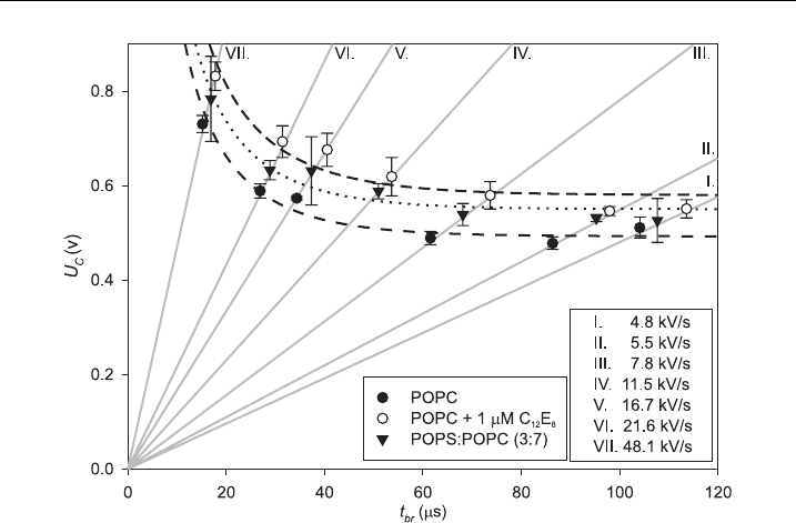
Figure 4 The breakdown voltage (U
c
) (dots) of lipid bilayers as a function of lifetime t
br
.The
gray l ine s show seven di¡erent slopes (k) of applied liner rising voltage signal. Dash, dotted and
dash^dotted curves represe nt two parameters curve ¢tted to data (1). Asymptotes of the curves (a)
correspond to minimal breakdown voltage U
cMIN
for lipid bilayers made of POPC, POPC+1 mM
C
12
E
8
and POPS:POPC (3:7) (Table 3).
M. Pavlin et al.174

the amplitude of fluctuations varied in a rather broad interval (form 150 to 1500 pS)
and they related them with the formation of local conductive defects (see theo-
retical explanations in the next chapter).
Robello et al. [52] observed a sharp increase in conductance induced by external
electric field obtained under current clamp conditions. They related it with cre-
ation of hydrophilic paths that increase the planar lipid bilayer conductance by one
order of magnitude.
Similarly Kalinowski et al. [70] presented chronopotentiometric method for
following planar lipid bilayer conductance during local conductive defects creation
that also allows observing of their dynamical behavior. The voltage fluctuations
reported in their work are consistent with theoretical models that predict formation
of temporary aqueous pathways across the membrane.
3. Attempts of Theoretical Explanation of
Electroporation
A number of theoretical models have been put forward as possible explana-
tions of electroporation. Here, an attempt will be made to present these models
roughly in their chronological order of appearance, and to review them critically,
Table 3 Capacitance of planar lipid bilayers measured by various methods in dierent salt
solutions.
BLM C (mF/cm
2
) Salt solution Method Reference
Azolecitin 0.59 0.1 M KCl Discharge pulse [38]
0.3–0.4 – Current ramp [69]
DOPC 0.1 M NaCl Discharge pulse [41]
DOPE 0.1 M NaCl Discharge pulse [41]
DPh PC 0.60–0.75 0.1 M KCl [51–53,55]
0.76–1.13 1 M KCl [51,54]
0.36 1 M NaCl Discharge pulse [41]
Ox Ch 0.555 1 M KCl Discharge pulse [41]
0.5 Current ramp [69]
0.41 1 M KCl Muxd sin wave [59]
0.45 0.1 M KCl Muxd sin wave [68]
0.47 0.5 M KCl Muxd sin wave [68]
0.40 1 M KCl Muxd sin wave [68]
PC 0.75 0.1 M KCl Current clamp triangular [52,55]
PI 0.25 1 M KCl Muxd sin wave [59]
0.30 0.1 M KCl Muxd sin wave [68]
0.27 0.5 M KCl Muxd sin wave [68]
0.25 1 M KCl Muxd sin wave [68]
POPC 0.59 0.1 M KCl Discharge pulse [37]
Electroporation of Planar Lipid Bilayers and Membranes 175

comparing their properties and abilities to those that the complete theoretical
description of electroporation should provide:
A physically realistic picture of both the nonpermeabilized and the permeabili-
zed membrane. Unlike a true breakdown process, electroporation does not lead
to a total disintegration of the system, but is localized and often even reversible.
Limited reversibility. Based on the amplitude and duration of electric pulses, the
permeabilized state is either reversible or irreversible.
Dependence on pulse duration and the number of pulses. With longer pulses, a
lower amplitude suffices for achieving the permeabilized state.
A realistic value of the minimal transmembrane voltage (‘‘critical voltage’’)
at which permeabilization occurs. Most of the presented models provide an
expression for this voltage, typically a function of several quantities. By inserting
the typical values of these quantities into the expressions, we assess their agree-
ment with experimentally measured critical voltage, which is in the range of a
few hundred millivolts. These values are given in Table 4, where those which are
either known only up to an order of magnitude, or can vary considerably, are
marked by a tilde.
Stochasticity. Variability of the critical pulse amplitude in experiments on cells
can largely be attributed to the variability of cell size within the treated pop-
ulation. However, a certain degree of stochasticity is also observed in elect-
ropermeabilization of pure lipid vesicles and planar bilayers. Some authors view
the ability of a model to account for this as crucial [32].
Table 4 Values of the quantities used in the evaluation of the models.
Parameter Notation Value Reference or
explanation
Membrane
Electric conductivity s
m
3 10
7
S/m [71]
Dielectric permittivity e
m
4.4 10
11
F/m [71]
Elasticity module Y 1 10
8
N/m
2
[72]
Viscosity m 0.6 Ns/m
2
[73]
Surface tension G 1 10
3
J/m
2
[32]
Edge tension g 1 10
11
J/m [32]
Thickness (undistorted) d
0
5 10
9
m [1]
Cytoplasm
Electric conductivity s
i
0.3 S/m [74,75]
Dielectric permittivity e
i
7.1 10
10
F/m Set at the same value
as e
e
Extracellular medium
Electric conductivity s
e
1.2 S/m [76] (blood serum at
351C)
Dielectric permittivity e
e
7.1 10
10
F/m [77] (physiological
saline at 351C)
M. Pavlin et al.176
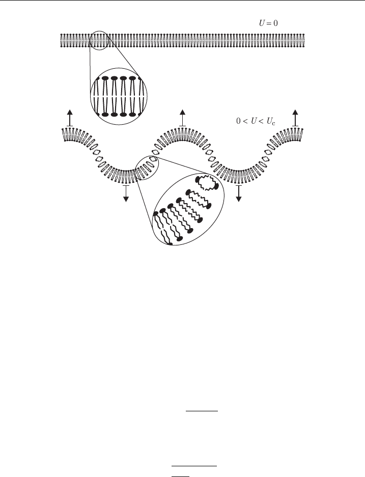
3.1. The Hydrodynamic Model
The hydrodynamic model, developed in the early 1970s [78,79], describes the
membrane as a charged layer of a nonconductive and noncompressible liquid sep-
arating two conductive liquids. The transmembrane voltage exerts a pressure on this
layer, and as it is assumed noncompressible in volume, the decrease in its thickness
leads to an increase in its surface area. If either the volume enveloped by the
membrane (in vesicles) or the perimeter of the membrane (in planar bilayers) is
assumed to remain constant, the membrane thus becomes rippled (Fig. 5).
As the membrane surface area increases, so does its surface tension and thereby
the pressure opposing the compression. At sufficiently low voltages, the two pressures
reach an equilibrium at which the membrane thickness stabilizes. However, as shown
in Appendix A.1, this equilibration is only possible up to the critical voltage given by
U
c
¼
ffiffiffiffiffiffiffiffi
Gd
0
2
m
r
(2)
where G is the surface tension of the membrane, d
0
its uncompressed thickness and
e
m
its dielectric permittivity. Above U
c
an instability occurs: the compressive pressure
prevails, causing a breakdown of the membrane. Applying typical parameter values
from Table 4 to the above expression, we get U
c
E0.24 V, which is in good agree-
ment with the experimental data. The equations in Appendix A.1 also describe the
membrane thickness as a function of the transmembrane voltage (Fig. 6).
The hydrodynamic model has several shortcomings. First, it applies to liquids
with isotropic fluidity, which is not true for lipid bilayers, where transverse move-
ment of molecules is very restricted. Second, it fails at the very first requirement
listed at the beginning of this chapter, as it does not describe the permeabilized
Figure 5 Membrane deformation accordi ng to the hydrodynamic model.
Electroporation of Planar Lipid Bilayers and Membranes 177

membrane. Of the other requirements, only the prediction of a realistic critical
transmembrane voltage is met.
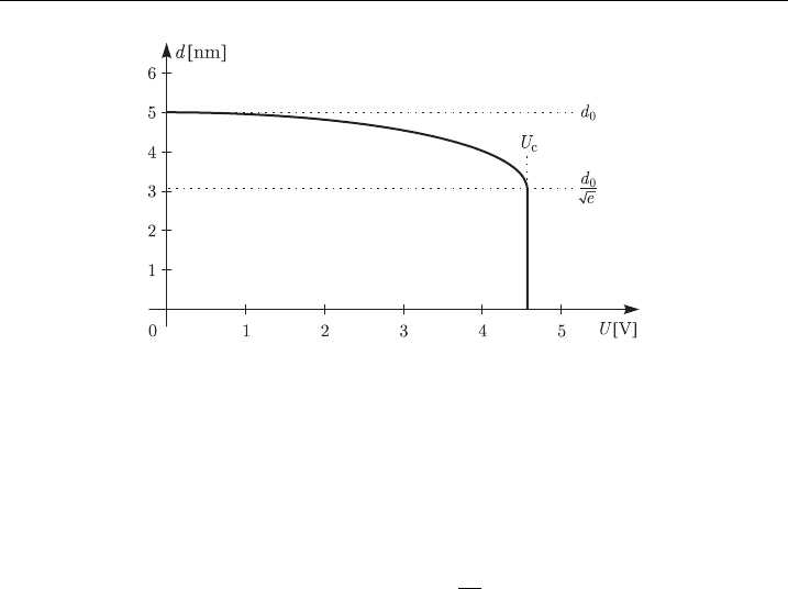
3.2. The Elastic Model
In contrast to the hydrodynamic model, which assumes a membrane with a con-
stant volume and a variable surface, the elastic model, presented soon afterwards
[80], assumes a variable volume and a constant surface (Fig. 7). In the elastic model,
Figure 6 Membrane thickness as a function of the transmembrane voltage in the hydrodynamic
model, usi ng parameter values fromTable 4.
Figure 7 Membrane deformation according to t he elastic model.
M. Pavlin et al.178
the pressure exerted by the transmembrane voltage leads to a decrease in the volume
of the membrane and an increase of elastic pressure opposing the compression. Also
here, the equilibrium becomes impossible above a critical voltage (see Appendix
A.2) given by
U
c
0:61 d
0
ffiffiffiffiffi
Y
m
r
(3)
where Y is the elasticity module of the membrane, d
0
its uncompressed thickness
and e
m
its dielectric permittivity. Above U
c
, there is an instability similar to the one
in the hydrodynamic model.
Applying typical parameter values (Table 4) to the expression above, we get
U
c
E4.57 V, which is roughly an order of magnitude too large. With the equations
in Appendix A.2, we can also plot the membrane thickness as a function of the
transmembrane voltage (Fig. 8).
In addition to the unrealistic prediction of critical voltage, the model assumes
that Y does not vary with deformation, which is certainly false at 39% compression
of the membrane at the point of instability (Fig. 8). This model also offers no
description of the permeabilized membrane, and fails to meet any other require-
ment listed at the beginning of this chapter.
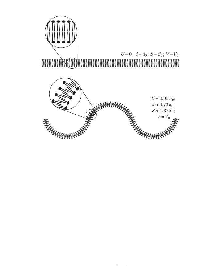
3.3. The Hydroelastic Model
The assumptions on which the hydrodynamic and the elastic model are built are
mutually excluding as well as unrealistic. By treating the membrane as a liquid with
both surface tension and elasticity, one obtains the more realistic hydroelastic
model, in which both the volume and the surface of the membrane vary, and the
charged membrane both compresses in volume and forms ripples (Fig. 9).
Similarly to the two models described previously, the hydroelastic model pre-
dicts a compressive instability (see Appendix A.3). With typical parameter values
(Table 4) it yields U
c
E0.34 V, which is in good agreement with experimental data.
Figure 8 Membrane thickness as a function of the transmembrane voltage in the elastic model,
using parameter values fromTa b l e 4.
Electroporation of Planar Lipid Bilayers and Membranes 179

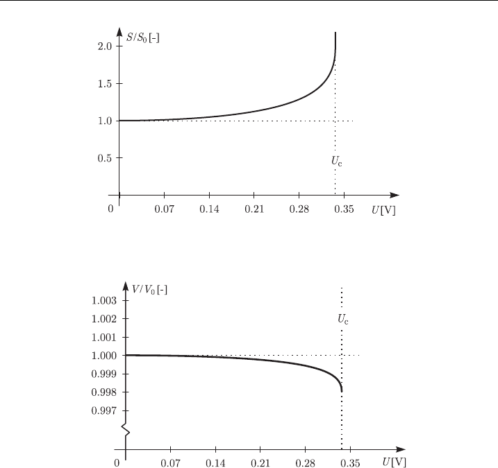
According to the hydroelastic model, at U
c
the membrane thickness is reduced to
50% of the initial value (Fig. 10), its surface is enlarged to almost 200% of the initial
value (Fig. 11) and the volume is reduced to 99.8% of the initial value (Fig. 12).
As Fig. 12 shows, according to the hydroelastic model the volume compression
is very small, and even at the critical voltage the membrane volume is reduced by
only 0.2% with respect to the initial value. Therefore, in this model the assumption
of constant value of the elasticity module is much more reasonable than in the
elastic model, in which the membrane breakdown is associated with a volume
reduction of almost 39%. While the description of the compressive instability
provided by the hydroelastic model is more realistic than those of the hydrodynamic
Figure 9 Membrane deformation according to the hydroelastic model.
Figure 10 Membrane thickne ss a s a function of the transmembrane voltage in the hydroelastic
model, usi ng parameter values fromTable 4.
M. Pavlin et al.180
and the elastic model, it has the same general drawback – it gives a nonsensical
picture of the electropermeabilized membrane: a uniform, infinitely thin layer, only
this time a rippled one. With the exception of a realistic prediction of the critical
transmembrane voltage, the model also fails to meet any other requirement given in
the list at the beginning of this chapter.
3.4. The Viscohydroelastic Model
Making another step toward complexity, the viscohydroelastic model (referred to
by its authors as viscoelastic) expands the hydroelastic model by adding to it the
membrane viscosity [81,82]. As in the hydroelastic model, in this model the
charged membrane is both compressed and rippled. However, the viscosity impedes
the molecular flow, and thus the compression is not instantaneous, but follows the
onset of the transmembrane voltage gradually.
During the compression and rippling of the membrane, the impeded molecular
flow leads to the thinning of the membrane at those locations where the flow would
Figure 11 Membrane surface area as a function of the transmembrane voltage in the
hydroelastic model, using parameter values fromTab l e 4.
Figure 12 Membrane volume as a function of the transmembrane voltage in the hydroelastic
model, usi ng parameter values fromTa b l e 4.
Electroporation of Planar Lipid Bilayers and Membranes 181
have to be the most rapid to maintain the uniform thickness (Fig. 13). Up to a
certain voltage, the membrane still reaches a state of equilibrium, but at higher
voltages, the integrity of the membrane cannot be sustained and discontinuities
form at the locations of the highest thinning. The analysis of such instability is
elaborate and is described in more detail elsewhere [73,83], while Appendix A.4
gives a short outline of its results. This analysis shows that in the viscohydroelastic
model, the instability occurs if the transmembrane voltage exceeds the critical
amplitude given by
U
c
¼
ffiffiffiffiffiffiffiffiffiffiffiffiffiffi
8 GYd
3
0
2
m
4
s
(4)
and lasts longer than the critical duration,
t
c
¼
24m
2
m
U
4
Gd
3
0
8Y
(5)
where m is membrane viscosity, the rest of the notation being the same as in the
previously described models. Applying typical parameter values (Tabl e 4), we get
U
c
E2.68 V, so in this aspect the viscohydroelastic model performs worse than both
the hydroelastic and the hydrodynamic model. However, it also offers a principal
advantage over any of the previously described models, as the requirement of an
above-critical voltage is linked to that of above-critical duration, providing a pos-
sible explanation of the dependence of permeabilization on the duration of electric
Figure 13 Membrane deformation according to the viscohydroelastic model.
M. Pavlin et al.182
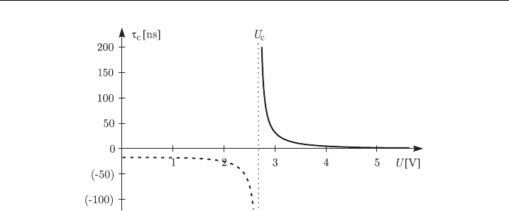
pulses. This is elucidated by Fig. 14, which shows the relation between the am-
plitude and the critical duration of the transmembrane voltage. At
U ¼ 1.01 U
c
E2.71 V, the critical duration t
c
of the transmembrane voltage is
approximately 450 ns, which is in close agreement with the sub-microsecond im-
aging experiments [84,85]. Still, the critical duration in the model decreases
extremely rapidly, and at U ¼ 1.20 U
c
E3.12 V we already have t
c
E17 ns, while
experimentally this decrease is much slower. Also, according to the viscohydro-
elastic model, the permeabilized membrane is torn along the ripples, but no such
disconnections have so far been observed, making this description of the perm-
eabilized membrane questionable.
3.5. The Phase Transition Model
According to the models presented up to this point, electropermeabilization is a
modification of the supramolecular membrane structure. In contrast, the phase
transition model describes this phenomenon as a conformational change of mem-
brane molecules [72]. On the molecular scale, the pressures are replaced by mo-
lecular energies, and the pressure equilibrium corresponds to the state of minimum
free energy. With several minima of free energy, several stable states are possible,
each corresponding to a distinct phase. In lipid bilayers, there are in general two
such phases, solid (gel) and liquid phase.
The phase transition model of electropermeabilization is an extension of the
statistical mechanical model of lipid membrane structure [86,87]. According to this
model, the free energy of the membrane at a temperature T and an average mo-
lecular surface area S is given by an expression of a general form
W ðT; SÞ¼W
f
ðSÞþW
c
ðT; SÞþW
ic
ðT; SÞþW
ih
ðT; SÞ (6)
where W
f
is the flexibility energy (from continuous deformations, e.g. compres-
sion), W
c
is the conformational energy (from discrete deformations, e.g. trans–cis
transitions), W
ic
is the energy of interactions between the hydrocarbon chains and
W
ih
is the energy of interactions between the polar heads of the lipids. Regrettably,
Figure 14 Critical duration of the transmembrane voltage as a function of its amplitude in the
viscohydroelastic model, using parameter values f romTable 4.
Electroporation of Planar Lipid Bilayers and Membranes 183