Lewis R.I. Turbomachinery Performance Analysis

164

Vorticity production in turbomachines and its influence upon meridional flows

and introducing Eqns (6.58)

dp

C r ~p C x @

dn Cs Ox Cs Or

Thus finally, the compressibility terms on the right-hand side of the governing

equation (6.57) become

@ @ dp

It is useful to note here that the operator

--Cr(O/OX ) "1-

Cx(O/Or)

performs the differential

of a quantity normal to the meridional streamlines d/dn multiplied by the meridional

velocity G. The governing equation (6.57) for compressible meridional flow now

becomes

a2r 1 ar s dp

ax 2 r ar ~- ~r 2 = - Prt~176 + rcs-~n

(6.59)

Another important result follows from a reconsideration of EqrL (6.17) for compres-

sible flow. Thus

ar ar

dd/= dx + dr

Ox ar

= -- prcrdx -t- prcx dr

Introducing Eqns (6.58) this transforms into

de = prcs(-dx

sin a + dr cos a)

= prcs(dn

sin 2 a + dn

COS 2 a) --

prcs dn

Thus finally the meridional velocity

Cs

is given by

Cs "--

1 d~

pr dn

(6.60)

For numerical computation Eqn (6.59) could be rewritten more conveniently

s

lar s d~ ldp

~m

Ox 2 r Or t- ~ = - pno o + dn p dn

(6.61)

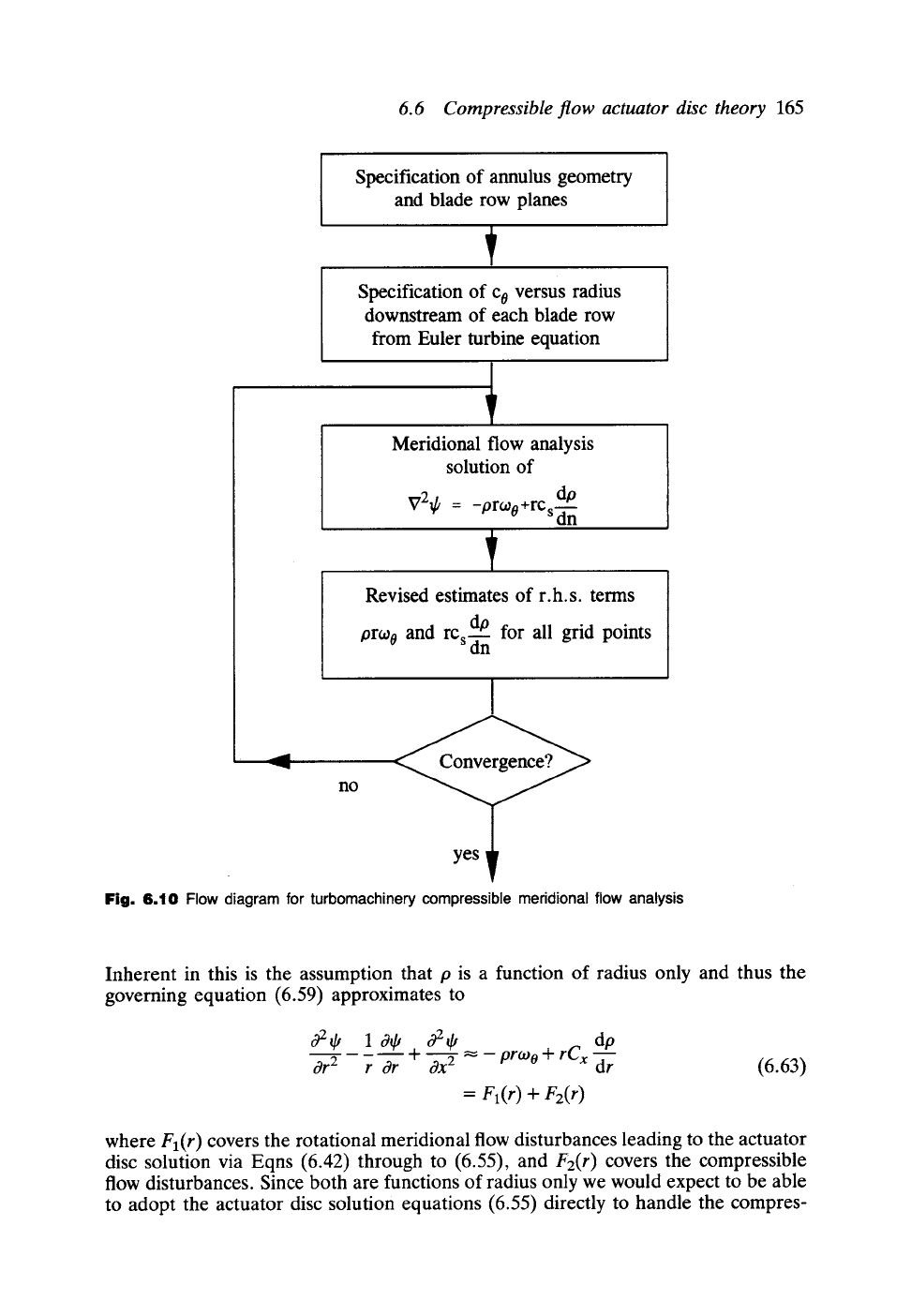
A full numerical analysis would thus require an iterative process such as that illustrated

in Fig. 6.10. Alternatively for cylindrical annuli we could make the linearising

assumption that the compressible term in Eqn (6.59) may be approximated to

dp dp

rCs -~n "~ rCx ~

(6.62)

6.6 Compressible flow actuator disc theory

165

Specification of annulus geometry

and blade row planes

Specification of c o versus radius

downstream of each blade row

from Euler turbine equation

Meridional flow analysis

solution of

do

V2t]' =

-Pr~176

+rCs

d'n

Revised estimates of r.h.s, terms

and rCs dp for all grid points

prco o

tin

I

no

Fig.

6.10 Flow diagram for turbomachinery compressible meridional flow analysis

Inherent in this is the assumption that p is a function of radius only and thus the

governing equation (6.59) approximates to

s162

1

0r s162 dp

ar 2 r ar 4- ~x 2 ~ - prto o + rCx -~r

(6.63)

= Fl(r)+ Fz(r)

where

Fl(r)

covers the rotational meridional flow disturbances leading to the actuator

disc solution via Eqns (6.42) through to (6.55), and F2(r) covers the compressible

flow disturbances. Since both are functions of radius only we would expect to be able

to adopt the actuator disc solution equations (6.55) directly to handle the compres-

166

Vorticity production in turbomachines and its influence upon meridional flows

sible flow problem. Although this is possible, a more direct analysis, offering also

deeper perception of the physical nature of compressible flows, follows from adoption

of the velocity potential instead of the stream function. This will be introduced in

the next section.

6.6.2 Analogy between compressible flows and incompressible flows with source

distributions

The continuity equation in vector form has already been stated as follows:

div p~ = 0 Compressible flow 1 [6.4]

div ~ = 0 Incompressible flow

J

The equation for incompressible flow may be further developed to accommodate

spatial distributions of source strength S, defined as fluid created at any point per

unit volume per unit time. Equation (6.4b) then becomes

div ~ = S (6.64)

An analogy with compressible flow follows if the vector derivative of Eqn (6.4a) is

expanded, namely

div p~ = p div ~ + ~. grad p = 0

Rearranging this, the compressible ftow continuity equation may be expressed as

1

div~ : ---~.gradp

(6.65)

P

=or

The quantity on the right-hand side,

-(1/p)~.gradp,

which absorbs all of the

compressibility effects could be treated analytically as an equivalent distributed source

density or in incompressible flow; thus Eqns (6.64) and (6.65) are identical in form.

In the one case the Poisson term S is due to distributed source strength. In the other

case the Poisson term or is caused by local gradients of fluid density.

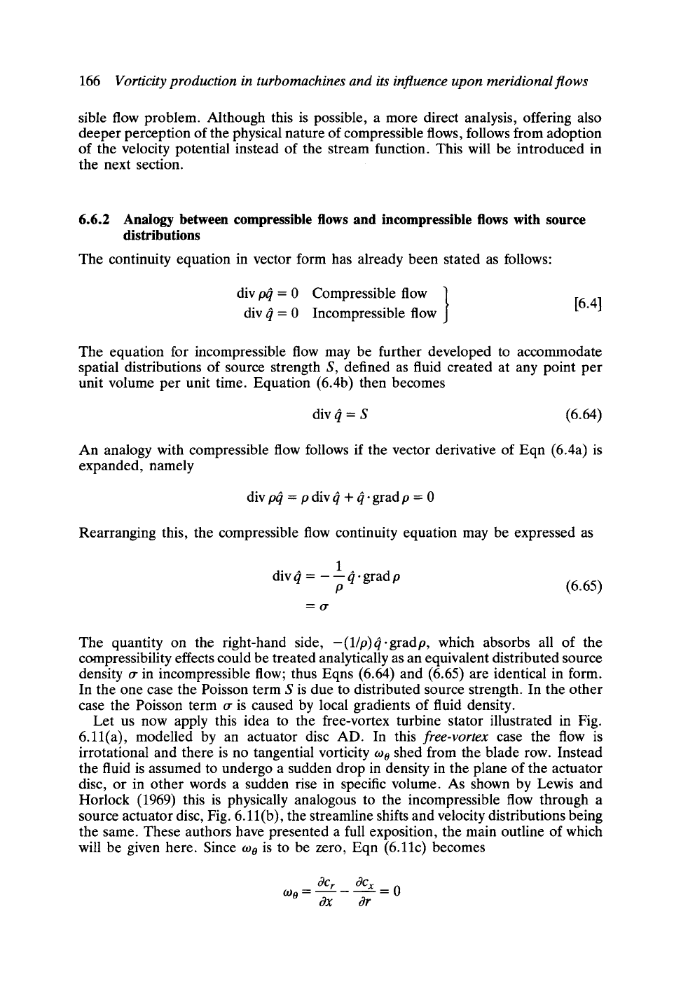
Let us now apply this idea to the free-vortex turbine stator illustrated in Fig.

6.11(a), modelled by an actuator disc AD. In this

free-vortex

case the flow is

irrotational and there is no tangential vorticity too shed from the blade row. Instead

the fluid is assumed to undergo a sudden drop in density in the plane of the actuator

disc, or in other words a sudden rise in specific volume. As shown by Lewis and

Horlock (1969) this is physically analogous to the incompressible flow through a

source actuator disc, Fig. 6.11 (b), the streamline shifts and velocity distributions being

the same. These authors have presented a full exposition, the main outline of which

will be given here. Since too is to be zero, Eqn (6.11c) becomes

tgC r aC x

s ~ 0

ox ar

6.6 Compressible flow actuator disc theory

167

f-

(a)

A

L

Cr

: t_.cx

A Source disc S(r)

f-

D

Co)

Fig. 6.11 Analogy between (a) compressible irrotational meridional flow through an axial turbine

free-vortex stator and (b) flow through an equivalent source actuator disc AD

which implies the existence of the velocity potential function th(x,r) such that

ar ar

Cx=~

and Cr=

ax Or

(6.66)

The continuity equation (6.65) then becomes

1

div grad ~b = or = - -- ~. grad p

P

or for axisymmetric flow

s 10~h

Ox2 +-

r gJr

t~2 t~ C x O~ p C r O~p

+ '~- =

pax p Or

c s dp

= S(x, r)

pds

(6.67)

where use has been made of Fig. 6.9 to establish the operator on the right-hand side,

cs(dp/ds) = Cx(Op/Ox)-t-Cr(Op/Or). S(x,r)

is the distributed source strength of the

equivalent incompressible flow. The physical meaning of this is that the compressible

flow disturbances are caused when the density changes along the direction of the

meridional velocity

Cs.

For a turbine

dp/ds

will assume large values due to flow

acceleration within the blade row. Elsewhere upstream and downstream of the stator

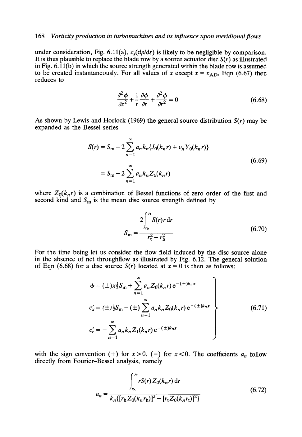
168

Vorticity production in turbomachines and its influence upon meridional flows

under consideration, Fig. 6.11(a),

cs(dp/ds)

is likely to be negligible by comparison.

It is thus plausible to replace the blade row by a source actuator disc

S(r)

as illustrated

in Fig. 6.1 l(b) in which the source strength generated within the blade row is assumed

to be created instantaneously. For all values of x except x =

XAO,

Eqn (6.67) then

reduces to

1 04) or

024) +- + = 0 (6.68)

ax 2 r ar

As shown by Lewis and Horlock (1969) the general source distribution

S(r)

may be

expanded as the Bessel series

oo

S(r)

= S m -

2 Z ankn{Jo(knr) + Vn Yo(knr)}

n--1

OQ

= S m ""

2 Z

anknZ~

n=l

(6.69)

where

Zo(kn r)

is a combination of Bessel functions of zero order of the first and

second kind and Sm is the mean disc source strength defined by

am -"

I rt

2 S(r)rdr

.'rh

rt

(6.70)

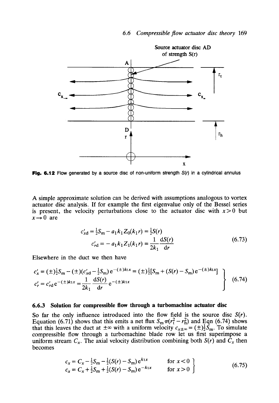
For the time being let us consider the flow field induced by the disc source alone

in the absence of net throughflow as illustrated by Fig. 6.12. The general solution

of Eqn (6.68) for a disc source

S(r)

located at x = 0 is then as follows:

oo

t~ = (_)x1Sm + Z

anZo(knr)e-(+-)knx

n--1

oo

Cx = (+)89 Z anknZ~

n--1

' Z

C r ~- -- anknZl(knr ) e-(+) k'x

n-1

(6.71)

with the sign convention (+) for x>0, (-) for x<0. The coefficients

an

follow

directly from Fourier-Bessel analysis, namely

an ---

frh

'trS(r) Zo(knr) dr

kn{[rh Zo(knrh)] 2 -

[rt

Zo(knrt)] 2}

(6.72)

6.6

A

Compressible flow actuator disc theory

169

Source actuator disc AD

of strength S(r)

C x -- ~ "~ ~ ._

Cx=

~ t.IJ ~ ~--

,..._

v

x

l r h

Fig. 6.12 Flow generated by a source disc of non-uniform strength

S(r)

in a cylindrical annulus

A simple approximate solution can be derived with assumptions analogous to vortex

actuator disc analysis. If for example the first eigenvalue only of the Bessel series

is present, the velocity perturbations close to the actuator disc with x>0 but

x---) 0 are

Cxd -" 89 -

alklZ0(kl r) =

89

1 dS(r)

Crd = -- alklZl(klr) = 2kl dr

Elsewhere in the duct we then have

(6.73)

CXcr == Cr d(-t-)lSm --e-(___)k,x(-F)(Cxd--lSm)e-(+--)klx==

2kl

I dS(r)dr

e-(___)kix

(-I-) l[Sm +

(S(r)-

Sm)e -(+)kax] }

(6.74)

6.6.3 Solution for compressible flow through a turbomachine actuator disc

So far the only influence introduced into the flow field is the source disc

S(r).

Equation (6.71) shows that this emits a net flux Sm 7r(r 2 -r 2) and Eqn (6.74) shows

that this leaves the duct at +oo with a uniform velocity

Cx+_~

= (+)lSm. To simulate

compressible flow through a turbomachine blade row let us first superimpose a

uniform stream

Cx.

The axial velocity distribution combining both

S(r)

and

Cx

then

becomes

Cx -- Cx - 1am -

l (S(r)

-

am)

e k'x

Cx = Cx d- 1S m Jr-

l (S(r)

-

am)

e -k'x

for x < 0 ~ (6.75)

for x>0

J

170

Vorticity production in turbomachines and its influence upon meridional flows

$1

A

1

D

S(r)

A

d c

)__~ o+dp Cx2

Cxl

c x +

dc x

o a

1 2

D

(a) (b)

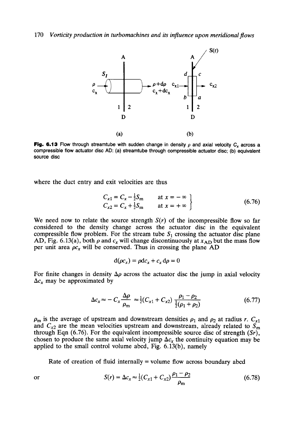
Fig. 6.13 Flow through streamtube with sudden change in density p and axial velocity

Cx

across a

compressible flow actuator disc AD: (a) streamtube through compressible actuator disc; (b) equivalent

source disc

where the duct entry and exit velocities are thus

Cxl = C x -ls

m at x = --~ ]

(6.76)

Cx2 = Cx + 1Sm at x = +

We need now to relate the source strength S(r) of the incompressible flow so far

considered to the density change across the actuator disc in the equivalent

compressible flow problem. For the stream tube $1 crossing the actuator disc plane

AD, Fig. 6.13(a), both p and Cx will change discontinuously at XAD but the mass flow

per unit area pCx will be conserved. Thus in crossing the plane AD

d(pcx) = pdcx + Cx dp = 0

For finite changes in density Ap across the actuator disc the jump in axial velocity

Acx may be approximated by

ACx ~ _ Cx Ap ~ l(Cx 1 q- Cx2) Pl - P2

(6.77)

Pm l(p 1 d-/92)

Pm is the average of upstream and downstream densities Pl and P2 at radius r. Cxl

and Cx2 are the mean velocities upstream and downstream, already related to Sm

through Eqn (6.76). For the equivalent incompressible source disc of strength (Sr),

chosen to produce the same axial velocity jump Acx the continuity equation may be

applied to the small control volume abcd, Fig. 6.13(b), namely

Rate of creation of fluid internally = volume flow across boundary abcd

or

S(r) = Acx-~

89 q- Cx2 ) Pl - P2

Pm

(6.78)

6.6 Compressible flow actuator disc theory

171

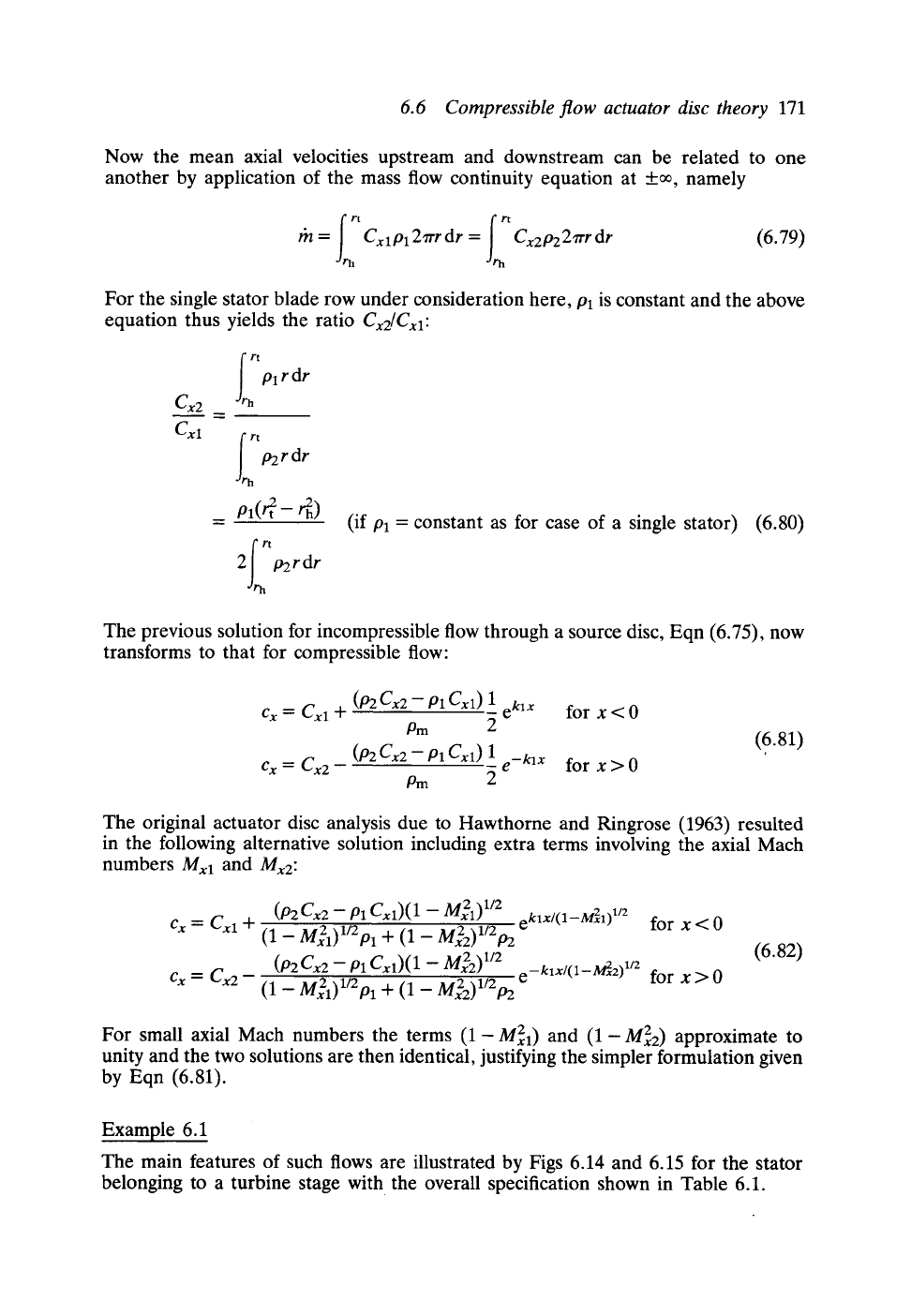
Now the mean axial velocities upstream and downstream can be related to one

another by application of the mass flow continuity equation at +oo, namely

I rt

& = CxlP127rrdr = Cx2P22zrrdr

h

(6.79)

For the single stator blade row under consideration here, Pl is constant and the above

equation thus yields the ratio

Cx2/Cxl"

Cx2

cxl

i rtpl r dr

h

i rtp2r dr

h

pl(/~t-/2h)

frh t

2 P2 r dr

(if Pl

=

constant as for case of a single stator)

(6.80)

The previous solution for incompressible flow through a source disc, Eqn (6.75), now

transforms to that for compressible flow:

Cx ._ Cx I +

(P2

Cx2- Pl

Cxl ) _1

ekax

for x < 0

Pm 2

Cx Cx 2 _

(P2

Cx2- Pl Cxl) 1 -klx

= -e for x>0

tim

2

(6.81)

The original actuator disc analysis due to Hawthorne and Ringrose (1963) resulted

in the following alternative solution including extra terms involving the axial Mach

numbers

Mxl

and

Mx2:

(p2Cx2- Pl

Cxl)(1

- M21) 1/2

eklX/(1_M21)1/2

Cx "~ Cxl +

(1

-

M21)1/2p1 +

(1

-

M22)1/2p2 for x < 0

(p2Cx2- Pl

Cxl)(1 - M22) 1/2

Cx = Cx2 -

(1

-

M21)1/2p1 -[-

(1

-/~x22)1/2p2

e -klx/(1-M2x2)1/2

for x > 0

(6.82)

For small axial Mach numbers the terms (1- M21) and (1-

M22)

approximate to

unity and the two solutions are then identical, justifying the simpler formulation given

by Eqn (6.81).

Example 6.1

The main features of such flows are illustrated by Figs 6.14 and 6.15 for the stator

belonging to a turbine stage with the overall specification shown in Table 6.1.

172

Vorticity production in turbomachines and its influence upon meridional flows

Table

6.1 Specification for model turbine stage

Hub/tip ratio

rh/r t

= 0.6

At r.m.s, radius:

Flow coefficient t~m "-0.5

Work coefficient q~m = 1.0

Exit Mach no. at rh, M2h = 1.0

Total to total efficiency r/Tr = 92%

Zero swirl upstream of stator

Free-vortex swirl distribution downstream of

stator

Perfect gas assumed with the properties of air

1.6

Cx

Cxl 1.4

[

1.2

0.8

-0.6 -0.4 -0.2 0.0

0:2 o14 0.6

x

I

~ hub

o

tip i

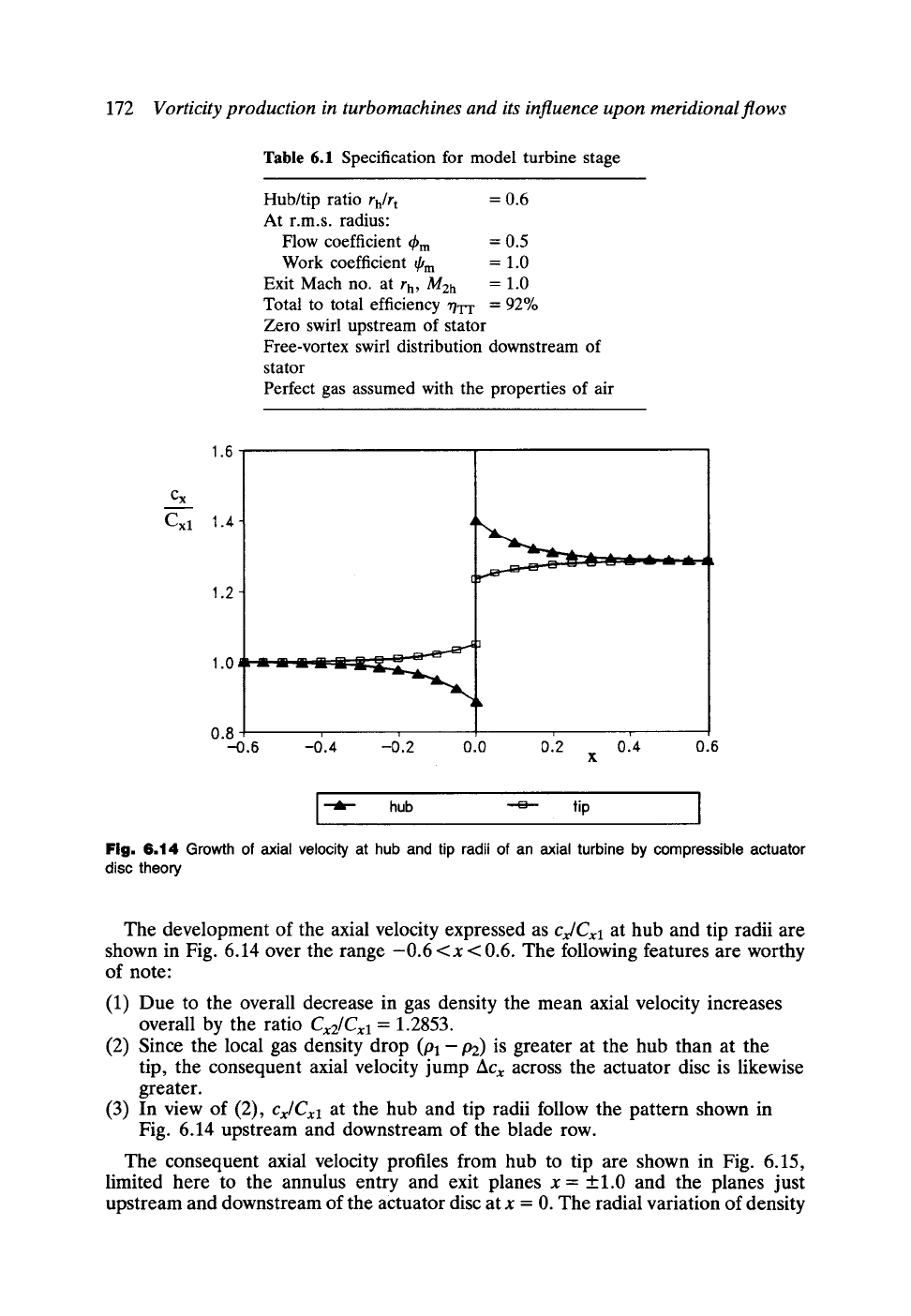
Fig. 6.14 Growth of axial velocity at hub

and tip radii of

an axial turbine by

compressible actuator

disc

theory

The development of the axial velocity expressed

as

Cx/fxl

at hub and tip radii are

shown in Fig. 6.14 over the range -0.6 <x < 0.6. The following features are worthy

of note:

(1) Due to the overall decrease in gas density the mean axial velocity increases

overall by the ratio

Cx2/C~I

= 1.2853.

(2) Since the local gas density drop (Pl- P2) is greater at the hub than at the

tip, the consequent axial velocity jump

ACx

across the actuator disc is likewise

greater.

(3) In view of (2),

cx/Cxl

at the hub and tip radii follow the pattern shown in

Fig. 6.14 upstream and downstream of the blade row.

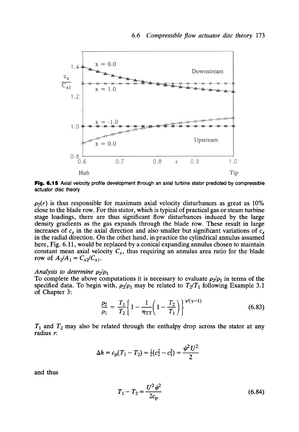
The consequent axial velocity profiles from hub to tip are shown in Fig. 6.15,

limited here to the annulus entry and exit planes x = +1.0 and the planes just

upstream and downstream of the actuator disc at x = 0. The radial variation of density

6.6 Compressible flow actuator disc theory

173

Fig. 6.15 Axial velocity profile development through an axial turbine stator predicted

by compressible

actuator disc theory

p2(r) is thus responsible for maximum axial velocity disturbances as great as 10%

close to the blade row. For this stator, which is typical of practical gas or steam turbine

stage loadings, there are thus significant flow disturbances induced by the large

density gradients as the gas expands through the blade row. These result in large

increases of

Cx

in the axial direction and also smaller but significant variations of

Cx

in the radial direction. On the other hand, in practice the cylindrical annulus assumed

here, Fig. 6.11, would be replaced by a conical expanding annulus chosen to maintain

constant mean axial velocity

Cx,

thus requiring an annulus area ratio for the blade

row of

A2/A1

= Cx2/Cxl.

Analysis to determine

P2/Pl

To complete the above computations it is necessary to evaluate

p2/Pl

in terms of the

specified data. To begin with,

P2/Pl

may be related to

T2/T1

following Example 3.1

of Chapter 3:

P2=pl T2TI[

1- r/Trl ( 1 -- TT~21 ) } v/(v-1) (6.83)

T1 and T2 may also be related through the enthalpy drop across the stator at any

radius r:

Ah = cp(T 1 - T2) = 89 4) =

2

and thus

T 1 - T 2 -- (6.84)

2Cp

Lewis R.I. Turbomachinery Performance Analysis

Подождите немного. Документ загружается.