Lee K.K. Lectures on Dynamical Systems, Structural Stability and Their Applications
Подождите немного. Документ загружается.

spectrum
ofT,
a(T).
Recall
that
the
set
of
linear
endomorphisms
of
B,
L(B),
is
a
Banach
space
with
the
norm
defined
by
ITI=
sup{IT(x)
I:
x e B,
lxl
S
1}.
And
the
spectrum
radius
r(T)
is
r(T)
=
sup{l~l:
~
E
a(T)}.
It
is
a
measure
of
the
eventual
size
of
T
under
repeated
iteration,
i.e.
,
it
equals
to
1
im.,._
IT"
1
11
".
One may
also
choose
a norm
of
B
such
that
T
has
norm
precisely
r(T)
with
respect
to
the
corresponding
norm
of
L(B).
When
r(T)
<
1,
we
call
T a
linear
contraction,
in
the
sense
of
metric
space
theory.
If
T
is
an
automorphism,
and
T"
1
is
a
contraction,
then
T
is
called
expansion.
Note
that
T
is
an
automorphism
iff
0
~
a(T),
and
that
r(T-
1
)
=
(inf
<1~1:
~
e
a(T)})-
1
•
In
fact,
a
(T"
1
)
= {
~-
1
:
~
E a
(T)
} •
Analogous
to
the
finite
dimensional
case,
let
GL(B)
be
the
open
subset
of
L(B)
consisting
of
all
linear
automorphisms
of
B.
LetT
e
GL(B),
and
if
a(T)
n s
1
is
empty,
then
we
call
T a
hyperbolic
linear
automorphism.
The
set
of
all
hyperbolic
linear
automorphisms
of
B
is
denoted
by
HL(B).
It
is
straightforward
to
show
that
if
T e
HL(B),
0
e B
is
the
only
fixed
point
of
T.
Now
let
D
be
a
contour,
symmetric
about
the
real
axis,
if
B
is
a
real
Banach
space,
such
that
a(T)
n D
is
empty.
Furthermore,
suppose
0
~
a(T)
and
that
D
separates
a(T)
into
two
subsets
a
5
(T)
and
au(T),
where
the
subscripts
sand
u
stand
for
stable
and
unstable
respectively,
as
we
shall
see
later.
Then
by
a
corollary
of
Dunford's
spectral
mapping
theorem,
B
splits
uniquely
as
a
direct
sum 8
5
+
Bu
of
T-invariant
closed
subspaces
such
that,
if
T
5
:
8
5
-+ 8
5
and
Tu:
Bu
-+
Bu
are
the
restrictions
of
T,
then
a (T
5
)
= a
5
(T)
and
a(Tu) =
au(T).
By
the
spectral
decomposition
theorem,
one
can
show
that
T
5
is
a
contraction
and
Tu
is
an
expansion.
Let
c
be
any
number
less
than
one
but
greater
than
the
larger
of
the
spectral
radii
of
T
5
and
Tu-
1
•
Then
one
can
prove:
Theorem
4.6.1
If
T E HL(B)
then
there
is
an
equivalent
norm
II II
such
that:
(i)
for
all
x = x
5
+
xu
E B,
llxll
=
max{
llxsll, llxull};
(ii)
max{ IITsll,
IITu-
1
11}
= a S
c.
Thus,
with
184
respect
to
the
new
norm
II
II,
T
8
is
a
metric
contraction,
and
Tu
is
a
metric
expansion.
The
stable
summand
B
8
of
B
with
rescect
to
T
is
characterized
as
(x
e B:
T"(x)
is
bounded
as
n
~
~
},
and
equivalently
as
(x
e
B:
T"(x)
~
0
as
n
~
~
}.
B
8
is
also
called
the
stable
manifold
of
0
with
respect
to
T,
and
T
8
is
called
the
stable
summand
of
T.
Similar
characterizations
and
definitions
hold
for
the
unstable
summand
B,
with
T-n
replacing
T".
We
say
that
T e HL(B)
is
isomorphic
to
T
1
e
HL(B
1
)
if
there
exists
a
topological
linear
isomorphism
from
B
to
B
1
taking
B
8
(T)
onto
B
8
1
(T
1
)
and
Bu
(T)
onto
Bu
1
(T
1
)
•
Equivalently,
T
is
isomorphic
to
T
1
iff
there
are
linear
isomorphisms
of
B
8
(T)
onto
B
8
1
(T
1
)
and
Bu(T)
onto
Bu
1
(T
1
).
Thus
there
are
exactly
n+1
isomorphism
classes
in
HL(R").
Theorem
4.6.2
HL(B)
is
open
in
GL(B),
and
hence
in
L(B).
Theorem
4.6.3
Any
T e HL(B)
is
stable
with
respect
to
isomorphism.
Theorem
4.6.4
Let
T
and
T
1
belong
to
the
same
path
component
of
GL(B)
and
also
have
spectral
radii
<
1.
Then
T
and
T
1
are
topologically
conjugate.
Corollary
4.6.5
Two
hyperbolic
linear
homeomorphisms
of
R"
are
topologically
conjugate
iff
(i)
there
are
isomorphic,
(ii)
their
stable
components
are
either
both
orientation
preserving
or
both
orientation
reversing,
and
(iii)
their
unstable
components
are
either
both
orientation
preserving
or
both
orientation
reversing.
Thus,
there
are
exactly
4n
topological
conjugacy
classes
of
hyperbolic
linear
automorphisms
of
R"
(n
~
1).
The
main
theorem
is:
Theorem
4.6.6
For
any
Banach
space
B,
any
T e HL(B)
is
stable
in
L(B)
with
respect
to
topological
conjugacy.
Corollary
4.6.7
Let
B
be
finite
dimensional,
then
HL(B)
is
the
stable
set
of
GL(B)
with
respect
to
topological
conjugacy.
Moreover,
HL(B)
is
an
open
dense
subset
of
GL(B).
Let
us
now
turn
to
study
linear
vector
fields.
We
are
185
interested
in
determining
which
vector
fields
are
stable
in
L(B)
with
respect
to
topological
equivalence.
We
call
T £
L(B)
a
hyperbolic
linear
vector
field
if
its
spectrum
a(T)
does
not
intersect
the
imaginary
axis
of
c,
and
we
denote
the
set
of
all
hyperbolic
linear
vector
fields
on
B
by
HLV(B).
Proposition
4.6.8
A
linear
vector
field
T
is
hyperbolic
iff
for
some
non-zero
real
t,
exp(tT)
is
a
hyperbolic
isomorphism.
Moreover,
T
has
integral
flow
¢:
RxB
~
B
given
by
¢(t,x)
=
exp(tT)(x).
As
before,
we
shall
define
stable
summands
and
stable
manifolds
at
o.
LetT£
HLV(B),
a
5
(T)
=
{~
£
a(T):
Re
~
< 0}
and
au(T)
=
{~
£
a(T):
Re
~
>
0}.
Also
let
D
be
a
contour
consisting
of
the
line
segment
(-ir,
ir]
and
the
semi-circle
{re;o
:
~12
S e S
3~/2}
where
r
is
large
enough
such
that
D
encloses
a
5
•
As
before,
the
spectral
decomposition
theorem
gives
a
T-invariant
direct
sum
splitting
B = 8
5
e
Bu
such
that
a(T
8
)
= a
8
(T)
and
a(Tu)
=
au(T),
where
T
5
£
L(B
5
)
and
Tu
£ L(Bu)
are
the
restrictions
of
T.
We
call
T
5
and
8
5
stable
summand
and
stable
manifold
at
0
respectively.
Likewise,
Tu
and
Bu
are
unstable
summand
and
unstable
manifold
at
0
respectively.
One
can
easily
show
that
for
all
t > o,
the
stable
summand
of
the
hyperbolic
automorphism
exp(tT)
is
exp(tT
5
)
and
similarly
for
unstable
summands.
One
can
show
that
the
map
exp:L(B)
~
L(B)
is
continuous,
and
since
HL(B)
is
open
in
L(B),
Proposition
4.5.8
implies
that
HLV(B)
is
also
open
in
L(B).
Moreover,
we
can
define
isomorphism
for
hyperbolic
vector
fields
just
as
for
hyperbolic
automorphisms.
Since
the
stable
and
unstable
summands
of
B
are
the
same
with
respect
to
T £ HLV(B)
as
with
respect
to
exp
T £ HL(B)
as
noted
before,
thus
T £
HLV(B)
is
stable
respect
to
isomorphism
follows
immediately
from
the
corresponding
result
for
HL(B).
We
then
have
the
following
theorem.
Theorem
4.6.9
LetT£
HLV(B),
then
T = T
5
e Tu,
where
a(T
8
) = a
8
(T)
and
a(Tu)
=
au(T).
The
set
HLV(B)
is
open
in
L(B),
and
its
elements
are
stable
with
respect
to
186
isomorphism.
As
in
the
case
of
hyperbolic
linear
automorphism,
we
may
choose
a
norm
on
B
such
that
the
stable
and
unstable
summands
of
exp(tT)
are
respectively
a
metric
contraction
and
a
metric
expansion.
Theorem
4.6.10
Let
T e HLV(B)
have
spectrum
a(T)
=
a
5
(T).
Then
there
exists
a
norm
1111
on
B
equivalent
to
the
given
one
such
that,
for
any
non-zero
x e
B,
the
map
from
R
to
(
0,
oo)
taking
t
to
II
exp
(tT)
(x)
II
is
strictly
decreasing
and
surjective.
There
also
exists
b > 0
such
that
for
all
t
>
O,
llexp(tT)
II
S
e·bt.
Corollary
4.6.11
If~:
RxB
~
B
is
the
integral
flow
of
T e
HLV(B),
then~
maps
RxS
1
homeomorphically
onto
B/{o}.
Theorem
4.6.12
Let
T,
T'e
HL(B)
have
spectra
in
Re
z <
o.
Then
T
and
T'
are
flow
equivalent.
Corollary
4.6.13
If
T
and
T'e
HLV(B)
are
isomorphic,
then they
are
flow
equivalent,
thus
topologically
equivalent.
Thus
we
have
the
following
important
result:
Theorem
4.6.14
Any
T e HLV(B)
is
stable
in
L(B)
with
respect
to
flow
equivalence,
thus
with
respect
to
topological
equivalence.
The
above
discussion
will
provide
the
basis
for
comparing
the
vector
field
or
flow
in
question
with
the
known
linear
vector
field
or
flow.
The
stable
and
unstable
decomposition
and
summands
are
the
basis
for
the
discussion
of
stability.
4.7
Linearization
As
we
have
pointed
out
earlier
we
can
hardly
expect
to
make
much
progress
in
the
global
theory
of
dynamical
systems
on
a
smooth
manifold
M,
if
we
ignore
completely
how
systems
behave
locally.
We
shall
attempt
to
classify
dynamical
systems
locally,
i.e.,
linearly.
But
even
here,
as
we
have
pointed
out
at
the
begining
of
section
5,
there
are
difficulties
with
linear
systems,
thus
we
can
only
expect
187
partial
success.
As
we
have
seen
earlier,
linear
systems
exhibit
a
diverse
variety
of
behavior
near
the
fixed
point
zero.
In
order
to
focus
on
our
classification
scheme,
we
shall
only
discuss
the
class
of
fixed
points
which
often
occurs
to
be
the
sort
that
one
"usually
comes
across".
For
linear
systems,
we
are
able
to
give
this
vague
notion
a
precise
topological
meaning
in
terms
of
the
spaces
of
all
linear
systems
on
a
given
Banach
space
B.
Let
¢
be
a
given
dynamical
system
on
a
smooth
manifold
M
which
has
a
fixed
point
p.
Since
we
are
only
interested
in
local
structure,
we
can
assume
M = B
and
p = o,
after
taking
a
chart
at
p.
Suppose
now
that
by
altering
¢
slightly
near
0
we
end
up
with
another
fixed
point
near
o,
with
a
local
phase
portrait
resembling
that
of
¢
at
o.
Intuitively,
the
linear
approximation
of
¢
at
0
(we
shall
make
sense
of
this
term
later)
must
have
a
phase
portrait
near
0
resembling
that
of
¢
near
0
as
most
all
"nearby"
linear
systems.
With
the
stability
theorems
of
the
last
section,
it
is
clear
that
we
should
consider
fixed
points
whose
linear
approximations
are
hyperbolic
systems.
A
fixed
point
p
of
a
diffeomorphism
f
of
M
is
hvDerbolic
if
the
tangent
map
TPf:
M
~
MP
is
a
hyperbolic
linear
automorphism.
Corollary
4.5.5
supplies
a
classification
of
hyperbolic
linear
automorphisms.
We
shall
extend
this
result
to
a
classification
of
hyperbolic
fixed
points
using
the
Hartman
theorem
[Hartman
1964;
Moser
1969]
which
states
that
any
hyperbolic
fixed
point
p
of
f
is
topologically
conjugate
to
the
fixed
point
0
of
TPf.
An
analogous
situation
exists
with
flows.
A
fixed
point
p
of
a
local
integral
¢:
IxU
~
M
of
a
vector
field
X
on
M
(or
equivalently
a
zero
of
X)
is
hyperbolic
if
for
some
t + 0
in
I,
p
is
a
hyperbolic
fixed
point
of
¢t
[Grobman
1959,
1962].
Proposition
4.7.1
The
point
p
is
a
hyperbolic
zero
of
a
vector
field
X
iff
for
any
chart
~
at
p,
the
differential
of
the
induced
vector
field
(T~)x~-
1
at
~(p)
is
a
hyperbolic
vector
field.
188
An
equivalent
but
more
sophisticated
approach
is
to
consider
TX:
TM
~
T(TM),
which
is
a
section
of
the
vector
bundle
T~":
T(TM)
~
TM,
where
~":
TM
~
M.
But
T~M
may
be
identified
with
the
tangent
bundle
on
TM,
where
~™:
T(TM)
~
TM
by
the
canonical
involution,
and
TX
then
becomes
a
vector
field
on
TM.
With
such
identification,
TPX
maps
MP
into
T(MP).
Thus
TPX
is
a
linear
vector
field
on
MP.
Recall
that
this
linear
vector
field
is
the
Hessian
of
X
at
p.
Thus:
Proposition
4.7.2
p
is
a
hyperbolic
zero
of
X
iff
the
Hessian
of
X
at
p
is
a
hyperbolic
linear
vector
field.
We
shall
state
later
that
if
p
is
a
hyperbolic
fixed
point
of
a
vector
field
X
then
it
is
flow
equivalent
to
the
zero
of
the
Hessian
of
X
at
p.
Recall
that
a
point
p
of
M
is
a
regular
point
of
a
dynamical
system
on
M
if
it
is
not
a
fixed
point
of
the
system.
The
following
two
theorems
show
that
regular
points
are
uninteresting
from
local
viewpoint.
Theorem
4.7.3
If
p
is
a
regular
point
of
a
diffeomorphism
f:
M
~
M
and
g
is
a
translation
of
the
model
space
B
of
M
by
a
non-
zero
vector
X
0
,
then
tip
is
topologically
conjugate
to
glo.
Theorem
4.7.4
Let
p
be
a
regular
point
of
a c
1
flow
~
on
M.
Let
x
0
be
any
non-zero
vector
of
the
model
space
B
of
M,
and
let
~·be
the
flow
on
B
defined
by
~(t,x)
= x +
tx
0
•
Then
~IP
is
flow
equivalent
to
~lo.
It
should
be
noted
that
the
equivalence
in
the
above
two
theorems
are
as
smooth
as
the
system
under
consideration.
Let
T
be
a
hyperbolic
linear
automorphism
of
B
with
skewness
a<
1
with
respect
to
the
norm I I
on
B,
i.e.,
max{ I T
8
I , I
Tn-
1
1 } = a <
1.
The
main
piller
of
the
theory
of
the
stability
of
T
with
respect
to
topological
conjugacy
under
smooth
small
perturbations
is
the
theorem
of
Hartman
[1964].
Lemma
4.7.5
Let~
: B
~
B
be
Lipschitz
with
constant
k
<
1-a.
Then
T+~
has
a
unique
fixed
point.
Theorem
4.7.6
(Hartman's
linearization
theorem)
Let
~
£ C
0
(B)
be
Lipschitz
with
constant
k < min{
1-a,
I T
5
"
1
1"
1
}.
189
Then
T+~
is
topologically
conjugate
to
T.
A
more
detailed
version
can
be
stated
as:
Theorem
4.7.7
Let~'
~
E C
0
(B)
be
Lipschitz
with
constant
k <
min{
1-a,
I T
5
"
1
1"
1
}.
Then
there
exists
a
unique
g
E C
0
(B)
such
that
(T+~)
(id+g)
=
(id+g)
(T+~).
Furthermore,
id+g
is
a
homeomorphism,
and
thus
is
a
topological
conjugacy
from
T+~
to
T+~.
Note
that,
the
conjugacy
id+g
in
the
above
theorem
cannot
always
be
as
smooth
as
T+~
or
T+~.
The
main
application
of
Hartman's
theorem
is
to
compare
a
diffeomorphism
near
a
hyperbolic
fixed
point
with
its
linear
approximation
at
the
point.
Corollary
4.7.8
A
hyperbolic
fixed
point
p
of
a c
1
diffeomorphism
f:
M
~
M
is
topologically
conjugate
to
the
fixed
point
o
of
TPf.
Corollary
4.7.9
There
are
4n
topological
conjugacy
classes
of
hyperbolic
fixed
points
that
occur
on
n-dimensional
manifolds.
In
relation
to
our
main
interest,
we
shall
say
a
few
words
concerning
stability.
We
call
a
fixed
point
p
of
a
diffeomorphism
f:
M
~
M
structurally
stable
if
for
each
sufficiently
small
neighborhood
U
of
p
in
M
there
is
a
neighborhood
V
of
f
in
Diff(M)
such
that,
for
all
g e V, g
has
a
unique
fixed
point
q
in
U
and
q
is
topologically
conjugate
to
p.
In
fact,
one
can
prove
that
fixed
points
are
structurally
stable
if
Cand
in
finite
dimensions.
only
if)
they
are
hyperbolic.
The
following
is
an
outline
of
the
proof.
Let
f:
U
~
f(U)
be
a
diffeomorphism
of
open
subsets
of
B
with
a
fixed
point
at
0
is
hyperbolic,
and
that
Df(O)
has
skewness
a
with
respect
to
the
norm
I I
on
B.
Choose
k,
where
0 < k <
1-a,
so
small
that
for
all
T e
L(B)
with
IT -
Df(O)
I S
k,
T
is
hyperbolic
and
topologically
conjugate
to
Df(O).
Let
Bb
be
a
closed
ball
in
B
with
center
o
and
radius
b
(<
1)
such
that
IDf(x)
-
Df(O)
I S
k/2
for
all
x e Bb.
Since
if~:
Bb
~
B
is
Lipschitz
with
constant
k
and
if
l~lo
S
b(1-a)
then
T+~:
Bb
~
B
has
a
unique
fixed
point.
One
can
190
prove
that
for
all
c
1
maps
g:
U
~
B
with
lg
-
fl
S
kb/2,
g
has
a
unique
fixed
point
p
in
~·
It
then
easily
follows
that
glp
is
topologically
conjugate
to
flo,
and
hence
0
is
structurally
stable
under
c
1
-small
perturbations
of
f.
Conversely,
one
can
prove
that
if
B
is
finite
dimensional
and
if
o
is
structurally
stable
under
c
1
-small
perturbation
of
f
then
o
is
hyperbolic.
Of
the
statement
we
have
just
outlined,
the
proof
is
a
very
important
one.
It
forms
a
basis
for
our
discussion
of
structural
stability
in
Chapter
6.
Let
us
now
discuss
Hartman's
linearization
theorem
in
the
context
of
flows.
It
was
discovered
independently
by
Grobman
[1959,1962].
Theorem
4.7.10
LetT
E
HL(B).
For
all
Lipschitz
maps
n
E C
0
(B)
with
sufficiently
small
Lipschitz
constant,
there
is
a
flow
equivalence
from
T
to
T+~.
Let
us
recall
the
definition
of
the
Hessian
of
a
map
at
a
critical
point.
Let
M
be
CO,
f
is
CO
on
M.
f
has
a
critical
point
at
p E M
if
dfP
= o.
If
p
is
a
critical
point
of
f,
then
the
Hessian
of
f
at
p,
Hf,
is
a
bilinear
function
on
MP
defined
as:
if
u,v
E
MP,
X E X(M)
such
that
if
X(p)
u,
then
Hf(u,v)
=
v(Xf).
Since
dfP
=
o,
then
HP(u,v)
is
independent
of
the
choice
of
X
and
Hf
is
symmetric.
With
Hessian
defined,
we
can
state
the
following
corollaries.
Corollary
4.7.11
A
hyperbolic
zero,
p,
of
a c
1
vector
field
on
M
is
flow
equivalent
to
the
zero
of
its
Hessian
at
p.
Corollarv
4.7.12
Flow
equivalence
and
orbit
equivalence
coincide
for
hyperbolic
zeros
of
c
1
vector
fields
on
an
n-dim.
manifold
M.
There
are
precisely
n+1
equivalence
classes
of
such
points
with
respect
to
either
relation.
Similar
to
the
statement
about
the
relationship
between
hyperbolic
fixed
point
and
structural
stability,
one
can
prove
the
following:
Let
X
be
a c
1
vector
field
on
B
with
a
zero
at
p.
If
p
is
hyperbolic
then
it
is
stable
with
respect
to
flow
equivalence
under
c
1
-small
perturbations
of
X.
Conversely,
if
B
is
finite
dim.
and
if
p
is
stable
with
191
respect
to
topological
equivalence
under
c
1
small
perturbation
of
X.
then
p
is
hyperbolic.
It
should
be
emphasized
that
hyperbolicity
of
fixed
points
is
not
an
invariant
of
topological
or
flow
equivalence.
In
other
words,
it
is
possible
for
a
non-hyperbolic
fixed
point
to
be
topological
or
flow
equivalent
to
a
hyperbolic
fixed
point.
For
instance,
the
non-hyperbolic
zero
of
the
vector
field
X(x)
= x
3
on
R
is
clearly
flow
equivalent
to
the
hyperbolic
zero
of
the
vector
field
W(x) =
x.
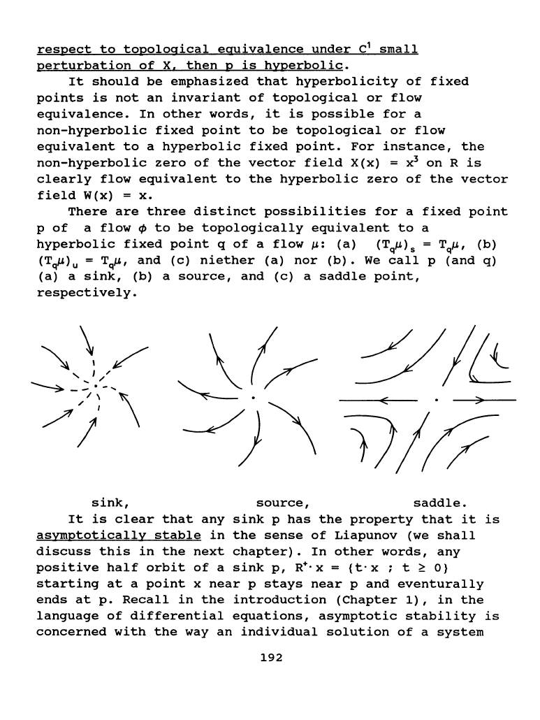
There
are
three
distinct
possibilities
for
a
fixed
point
p
of
a
flow
~
to
be
topologically
equivalent
to
a
hyperbolic
fixed
point
q
of
a
flow
iJ.:
(a)
(Tql-')
8
=
TqiJ.'
(b)
(Tql-')u
=
TqiJ.'
and
(c)
niether
(a)
nor
(b).
We
call
p
(and
q)
(a)
a
sink,
(b)
a
source,
and
(c)
a
saddle
point,
respectively.
"\.\/
' I ,
'
I'
~--·-
...
1\
\
/'/
sink,
~0~1~
__/)\
))//7
source,
saddle.
It
is
clear
that
any
asymptotically
stable
in
sink
p
has
the
property
that
it
is
the
sense
of
Liapunov
(we
shall
discuss
this
in
the
next
chapter).
In
other
words,
any
positive
half
orbit
of
a
sink
p,
R+·x =
(t·x
; t
~
0}
starting
at
a
point
x
near
p
stays
near
p
and
eventurally
ends
at
p.
Recall
in
the
introduction
(Chapter
1),
in
the
language
of
differential
equations,
asymptotic
stability
is
concerned
with
the
way
an
individual
solution
of
a
system
192
varies
as
the
initial
conditions
are
varied.
This
is
different
from
structural
stability,
which
deals
with
the
way
the
set
of
all
solutions
varies
as
we
change
the
system
itself.
It
is
appropriate
at
this
juncture
for
us
to
discuss
some
properties
of
hyperbolic
closed
orbits
and
Poincare
maps.
Let
p
be
a
point
on
a
closed
orbit
of
a cr
flow
~
(r
~
1)
on
a
manifold
M.
Suppose
that
the
orbit
r =
R·p
of~
through
p
has
period
r.
Then
~T:
M
~
M
is
a cr
diffeomorphism
with
p
its
fixed
point.
Where
the
tangent
map
TP~T
is
a
linear
homeomorphism
of
MP.
It
keeps
the
linear
subspace
<X(x)>
of
MP
pointwise
fixed,
where
X(x)
is
the
velocity
of
~
at
x,
because
~T
keeps
the
orbit
r
pointwise
fixed.
r
is
said
to
be
hyperbolic
if
MP
has
a
TP~T-
invariant
splitting,
i.e.,
MP
=
<X(p)>
e
FP
where
TP~TIFP
is
hyperbolic.
Thus,
hyperbolicity
for
a
closed
orbit
means
that
the
linear
approximation
to
~T
is
as
hyperbolic
as
possible.
A
clear
geometrical
picture
can
be
obtained
in
terms
of
Poincare
maps.
Let
N
be
some
open
disk
embedded
as
a
submanifold
of
M
through
p
such
that
<X(x)>
e
NP
=
~·
Notice
that
this
is
exactly
the
condition
of
transversality.
Indeed,
we
say
that
N
is
transverse
to
the
orbit
at
p,
and
call
it
a
cross-section
to
the
flow
at
p.
We
assert
that
for
some
small
open
neighborhood
U
of
p
in
N,
there
is
a
unique
continuous
function
p: U
~
R
such
that
P(p)
=
r,
and
~(p(y),y)
EN.
Here
pis
a
first
return
function
for
N.
Any
two
such
functions
agree
on
the
intersection
of
their
domains.
Intuitively,
p(y)
is
the
time
it
takes
a
point
starting
at
y
to
move
along
the
orbit
of
the
flow
in
the
positive
direction
until
it
hits
the
section
N
again.
We
denote
the
point
at
which
it
hits
again
by
f(y).
Thus,
f:
U
~
N
is
a
map
defined
by
f(y)
=
~(P(y),y).
193