Lee K.K. Lectures on Dynamical Systems, Structural Stability and Their Applications
Подождите немного. Документ загружается.

integral
of
a
vector
field
is
locally
a
flow.
Theorem
4.4.9
Let
~=
IxU
~
M
be
a
local
integral
of
a
locally
Lipschitz
vector
field
on
a
manifold
M.
Then
for
all
p e u
and
all
s,
t e I
such
that
s+t
e I
and
~(t,p)
e u,
~(s,~(t,p))
=
~(s+t,p).
It
follows
immediately:
Corollary
4.4.10
If
~=
IxM
~
M
is
a
local
integral
of
a
locally
Lipschitz
vector
field
on
a
manifold
M,
then
it
is
a
flow
on
M.
The
next
theorem
shows
the
uniqueness
of
an
integral
flow
in
a
Banach
space.
Theorem
4.4.11
Any
Lipschitz
vector
field
X
on
a
Banach
space
B
has
a
unique
integral
flow
~-
If
X
is
cr
then
~
is
also
cr.
The
next
theorem
shows
that
the
local
integrals
are
as
smooth
as
the
vector
field
we
integrate
and
this
is
completely
general.
Theorem
4.4.12
Any
local
integral
of
a cr
(r
~
1)
vector
field
on
a
manifold
M
is
cr.
Likewise,
any
integral
of
a
locally
Lipschitz
vector
field
is
locally
Lipschitz.
Theorem
4.4.13
Any
locally
Lipschitz
vector
field
X
on
a
compact
manifold
M
has
a
unique
integral
flow
~.
which
is
locally
Lipschitz.
If
X
is
cr
(r
~
1)
then~
is
also
cr.
By
virtue
of
the
fact
that
velocity
fields
and
integral
flows
are
so
closely
related,
the
qualitative
theories
of
smooth
vector
fields
and
smooth
flows
can
be
thought
of
as
one
and
the
same
subject.
Since
it
is
sometimes
easier
to
describe
the
qualitative
theory
in
terms
of
vector
fields,
and
at
other
times
in
terms
of
flow,
we
shall
feel
free
to
use
whichever
terminology
or
viewpoints
we
find
more
convenient
in
any
given
situation.
4.5
Dispersive
systems
In
Section
4.3
we
were
interested
in
the
systems
of
Poisson
stable
points
or
non-wandering
points,
and
recursiveness.
In
this
section,
we
shall
discuss
dynamical
174
systems
marked
by
the
absence
of
recursiveness.
We
shall
briefly
describe
dispersive
dynamical
systems
and
instability,
and
we
shall
also
study
the
theory
of
parallelizable
dynamical
systems.
First
we
shall
introduce
the
definition
of
positive
(negative)
prolongation
of
x e X.
For
any
x e X,
the
positive
(negative>
prolongation
of
x,
ot(x)
=
{y
e X:
there
is
a
sequence
{x"}
in
X
and
a
sequence
{tn}
in
Rt
such
that
xn
~
x
and
x"t"
~
y}.
The
positive
(negative)
prolongational
limit
set
of
x,
Jt(x)
=
{Y
e
X:
there
is
a
sequence
{X"}
in
X
and
a
sequence
{
t"}
in
Rt
such
that
xn
~
x,
tn
~
±
«J,
and
xntn
~
Y}
•
It
is
clear
that
for
any
x e X,
r±(x)
is
a
subset
of
o±(x),
n(x)
is
a
subset
of
J+(x),
a(x)
is
a
subset
of
J"(x).
These
inclusions
can
be
illustrated
by
considering
the
system,
dxjdt
=
-x,
dyjdt
=
y.
This
is
a
dynamical
system
with
a
saddle
point
at
the
origin.
We
will
leave
to
the
reader
to
graph
the
orbits
and
to
establish
the
above
inclusions.
Let
x e X,
and
the
partial
map
~x
is
positively
Lagrange
unstable
if
the
closure
of
the
positive
semi-orbits,
r+(x),
is
not
compact.
It
is
called
negatively
Lagrange
unstable
if
the
closure
of
r·(x)
is
not
compact.
And
it
is
called
Lagrange
unstable
if
it
is
both
positively
and
negatively
Lagrange
unstable.
In
Section
4.3
we
have
defined
Poisson
stable
and
wandering
points.
Now
we
are
ready
to
define
some
of
the
concepts
of
dispersiveness
of
a
dynamical
system.
A
dynamical
system
is,
Lagrange
unstable
if
for
each
x e
X
the
partial
map
~x
is
Lagrange
unstable,
Poisson
unstable
if
each
x
is
Poisson
unstable,
completely
unstable
if
every
x
is
wandering,
dispersive
if
for
every
pair
of
points
x,
y
e X
there
exist
neighborhoods
Ux
of
x
and
UY
of
y
such
that
Ux
is
not
positively
recursive
with
respect
to
UY.
As
an
example,
let
us
consider
a
dynamical
system
in
R
2
,
whose
phase
portrait
is
Fig.4.5.1.
The
unit
circle
contains
a
fixed
point
p
and
an
orbit
r
such
that
for
each
point
q e
r we
have
O(q)
=
a(q)
=
{p}.
All
orbits
in
the
interior
of
175

the
unit
circle
(=
{p}
U r)
have
the
same
property
as
r.
All
orbits
in
the
exterior
of
the
unit
circle
spiral
to
the
unit
circle
as
t
~
oo,
so
that
for
each
point
q
in
the
exterior
of
the
unit
circle
we
have
n(q)
=
{p}
U
r,
and
a(q)
=
o.
Notice
that
if
we
consider
the
dynamical
system
obtained
from
this
one
by
deleting
the
fixed
point
p,
now
the
dynamical
system
is
defined
on
R
2
-
{p},
then
this
new
system
is
Lagrange
unstable
and
Poisson
unstable,
but
it
is
not
completely
unstable
because
for
each
q E r
we
have
J•(q)
=
r,
i.e.,
q E
J+
(
q)
•
Fig.4.5.1
It
should
be
noted
that
for
dynamical
systems
defined
by
differential
equations
in
R
2
,
the
concepts
of
Lagrange
instability
and
wandering
are
equivalent.
This
may
be
easily
proven
by
using
the
Poincare-Bendixson
theorem
for
planar
systems.
Note
that
the
above
example
has
the
fixed
point
removed,
i.
e.
,
in
R
2
- {
p}
•
We
next
consider
an
example
of
a
dispersive
system
which
turns
out
to
be
not
parallelizable
when
we
introduce
this
concept
shortly.
Let
the
dynamical
system
in
R
2
be,
dxjdt
=
f(x,y),
dy/dt
= o,
where
f(x,y)
is
continuous,
and
f(x,y)
= 0
whenever
the
points
(x,y)
are
of
the
form
(n,ljn),
and
n
is
a
positive
176
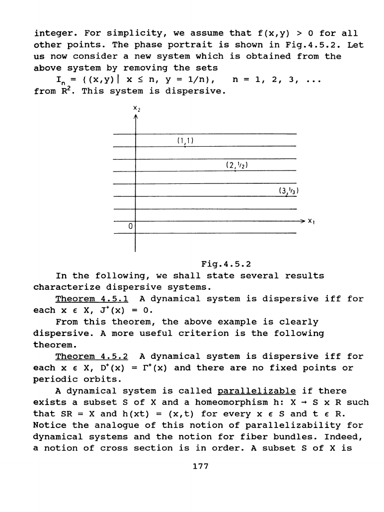
integer.
For
simplicity,
we
assume
that
f(x,y)
> 0
for
all
other
points.
The
phase
portrait
is
shown
in
Fig.4.5.2.
Let
us
now
consider
a
new
system
which
is
obtained
from
the
above
system
by
removing
the
sets
In
= { (
x,
y)
I x S
n,
y =
1/n}
, n =
1,
2 , 3 ,
•••
from
R
2
•
This
system
is
dispersive.
Xz
(1,1)
(2,
1
tz)
(3,
1
13)
0
Fig.4.5.2
In
the
following,
we
shall
state
several
results
characterize
dispersive
systems.
Theorem
4.5.1
A
dynamical
system
is
dispersive
iff
for
each
x € X,
J•(x)
=
o.
From
this
theorem,
the
above
example
is
clearly
dispersive.
A
more
useful
criterion
is
the
following
theorem.
Theorem
4.5.2
A
dynamical
system
is
dispersive
iff
for
each
x € X,
o•(x)
=
r•(x)
and
there
are
no
fixed
points
or
periodic
orbits.
A
dynamical
system
is
called
parallelizable
if
there
exists
a
subset
S
of
X
and
a
homeomorphism
h:
X
~
S x R
such
that
SR = X
and
h(xt)
=
(x,t)
for
every
x € s
and
t €
R.
Notice
the
analogue
of
this
notion
of
parallelizability
for
dynamical
systems
and
the
notion
for
fiber
bundles.
Indeed,
a
notion
of
cross
section
is
in
order.
A
subset
S
of
X
is
177
called
a
section
of
the
dynamical
system
if
for
each
x E X
there
is
a
unique
T(x)
such
that
xT(x)
E
s.
Note
that
not
every
dynamical
system
has
a
section.
In
fact,
any
dynamical
system
has
a
section
iff
it
has
no
fixed
points
or
periodic
orbits.
This
is
not
surprising,
because
from
the
fiber
bundle
view
point,
the
existence
of
a
section
implies
that
for
each
T(x),
continuous
or
not,
each
section
is
homeomorphic
to
each
other.
Note
also,
in
general
T(X)
is
not
continuous,
but
the
existence
of
a
section
s
with
continuous
T(x)
implies
certain
properties
of
the
dynamical
system.
Lemma
4.5.3
If
S
is
a
section
of
the
dynamical
system
with
T(x)
continuous
on
X,
then:
(i)
S
is
closed
in
X,
(ii)
S
is
connected,
arcwise
connected,
simply
connected
iff
X
is
connected,
arcwise
connected,
simply
connected
respectively,
(iii)
if
a
subset
K
of
s
is
closed
in
s,
then
Kt
is
closed
in
X
for
every
t E R,
(iv)
if
a
subset
K
of
S
is
open
in
s,
then
KI
is
open
in
X,
where
I
is
any
open
interval
in
R.
Theorem
4.5.4
A
dynamical
system
is
parallelizable
iff
it
has
a
sectionS
with
T(x)
continuous
on
X.
This
theorem
shows
that
the
dynamical
system
of
the
second
example
is
not
parallelizable.
The
next
theorem
is
a
very
important
one.
Theorem
4.5.5
A
dynamical
system
on
a
locally
compact
separable
metric
space
X
is
parallelizable
iff
it
is
dispersive.
The
proof
of
this
theorem
depends
on
certain
properties
of
sections.
We
shall
not
go
into
any
detail
here.
It
suffices
to
say
that
the
concept
of
tubular
neighborhoods
is
essential
to
its
development.
For
more
details,
the
reader
is
directed
to
Bhatia
and
Szeg6
[1970],
Ch.
4.
4.6
Linear
systems
Naively,
one
might
hope
to
obtain
a
complete
classification
of
all
dynamical
systems
on
Euclidean
space
R",
starting
with
the
simplest
types
and
gradually
building
178
up
some
understanding
of
more
complicated
ones.
The
simplest
diffeomorphisms
of
R"
are
translations,
and
it
is
easy
to
show
that
two
such
maps
are
linearly
conjugate
(topological
conjugate
by
a
linear
automorphism
of
R")
providing
the
constant
vector
is
non-zero.
Furthermore,
any
two
non-zero
constant
vector
fields
on
R"
are
linearly
flow
equivalent.
The
next
simplest
systems
are
linear
discrete
systems
generated
by
linear
automorphisms
of
R"
and
vector
fields
on
R"
with
linear
principal
part.
Even
more,
the
classification
problem
is
far
from
trivial,
nor
is
it
solved.
The
difficulties
one
encounters
even
with
linear
problems
underline
the
complexity
and
richness
of
the
theory
of
dynamical
systems.
And
indeed
this
is
a
major
part
of
its
attraction.
Meanwhile,
these
difficulties
also
indicate
the
need
for
a
modest
approach
to
the
problem.
We
only
attempt
to
classify
a
"suitably
large"
class
of
dynamical
systems
instead
of
the
complete
solution.
For
linear
systems
on
R",
it
is
easy
to
give
a
precise
definition
of
what
a
"suitably
large"
class
means.
The
set
L(R")
of
linear
endomorphisms
of
R"
is
a
Banach
space
with
the
norm
ILl=
sup{
IL(x)
I:
x £ R",
lxl=l}.
A
"suitably
large"
subset
of
linear
vector
fields
on
R"
is
the
one
both
open
and
dense
in
L(R").
Let
X
be
a
topological
space
and
-
is
an
equivalence
relation
on
X.
We
say
that
a
point
x £ X
is
stable
with
respect
to
-
if
x
is
an
interior
point
of
its
-
class.
The
stable
set
~
of
-
is
the
set
of
all
stable
points
in
X.
Clearly,
~
is
an
open
subset
of
X.
If
X
has
a
countable
basis,
then
~
contains
points
of
only
countably
many
equivalence
classes.
Nonetheless,
~
may
fail
to
be
dense
in
X.
In
the
present
context,
X=
L(R")
(or
GL(R")),
-is
topological
equivalence
(conjugacy),
and~
is
called
the
set
of
hyperbolic
linear
vector
fields
(automorphisms).
In
such
a
case,
~
is
dense
and
easily
classifiable.
The
basic
idea
of
calculus
is
to
approximate
a
function
locally
by
a
linear
function.
Similarly,
when
discussing
the
179
local
properties
of
a
dynamical
system
we
study
its
"linear
approximation",
which
is
a
linear
system.
The
important
question
is
whether
this
linear
system
is
a
good
approximation
in
the
sense
that
it
is
locally
qualitatively
the
same
as
the
original
system.
And
this
obviously
leads
to
the
stability
(in
the
broader
sense)
of
the
linear
system.
The
importance
of
considering
the
hyperbolic
linear
vector
fields
(automorphisms)
is
that
they
are
stable
not
only
under
small
linear
perturbations
but
also
under
small
smooth
(but
not
necessarily
linear)
perturbations.
We
shall
begin
with
a
review
of
linear
systems
on
R",
which
provide
a
background
of
concrete
examples
against
which
the
more
general
results
on
Banach
spaces
may
be
tested
and
placed
in
perspective.
Let
T
be
any
linear
endomorphism
of
R",
then
we
may
think
of
it
as
a
vector
field
on
R".
The
corresponding
ordinary
differential
equation
is
x'=
T(x)
where
x € R".
The
integral
flow
can
be
written
down
immediately.
Since
L(R")
is
a
Banach
space,
then
the
infinite
series
exp(tT)
=
id
+
tT
+
t•
T
2
/2
+
••••
+
t"T"/n!
+
•.•.
,
t €
R,
converges
for
all
t
and
T
and
the
integral
flow
~
of
Tis
~(t,x)
=
exp(tT)
(x).
We
shall
call
a
flow~
linear
if
~t
is
a
linear
automorphism
varying
smoothly
with
t.
Thus
~
is
linear
iff
its
velocity
field
is
linear.
As
an
example,
if
T =
a(id)
for
some a € R,
exp(tT)=
id
+
at(id)
+
••••
+
(at)"id"/n!
+
...
=
(1
+
at
+
•..
+
(at)"/n!
+
••
)
id
= e
8
tid.
A
notion
of
linear
equivalence
for
linear
flow
can
be
defined
by
letting
~
and
~
be
linear
flows
with
velocities
S
and
T € L(R")
respectively.
Then
~
is
linearly
equivalent
to
~,
~
"L
~,
if
for
some a €
R,
a > o,
and
linear
automorphism
h € GL(R")
of
R",
the
following
diagram
commutes:
R X R"
axh
~
R X R"
•
-+
-+
180
R"
~
h
R"
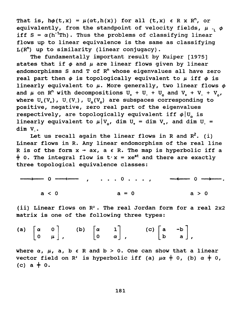
That
is,
h~(t,x)
=
~(at,h(x))
for
all
(t,x)
£ R x R",
or
equivalently,
from
the
standpoint
of
velocity
fields,
~
-L
~
iff
S =
a(h"
1
Th).
Thus
the
problems
of
classifying
linear
flows
up
to
linear
equivalence
is
the
same
as
classifying
L(R")
up
to
similarity
(linear
conjugacy).
The
fundamentally
important
result
by
Kuiper
[1975]
states
that
if
~
and
~
are
linear
flows
given
by
linear
endomorphisms
s
and
T
of
R"
whose
eigenvalues
all
have
zero
real
part
then
~
is
topologically
equivalent
to
~
iff
~
is
linearly
equivalent
to
~·
More
generally,
two
linear
flows
~
and
~
on
R"
with
decompositions
u. +
u_
+ U
0
and
v. +
V_
+ V
0
,
where
u.cv.), U_(V_), U
0
(V
0
)
are
subspaces
corresponding
to
positive,
negative,
zero
real
part
of
the
eigenvalues
respectively,
are
topologically
equivalent
iff
~IU
0
is
linearly
equivalent
to
~IV
0
,
dim
u.
=
dim
v.,
and
dim
U_
dim
v_.
Let
us
recall
again
the
linear
flows
in
R
and
R
2
•
(i)
Linear
flows
in
R. Any
linear
endomorphism
of
the
real
line
R
is
of
the
form
x
~
ax,
a £ R.
The
map
is
hyperbolic
iff
a
+ o.
The
integral
flow
is
t-x
=
xe•t
and
there
are
exactly
three
topological
equivalence
classes:
0 • 0 • •
. ,
0
a < o
a = 0
a > 0
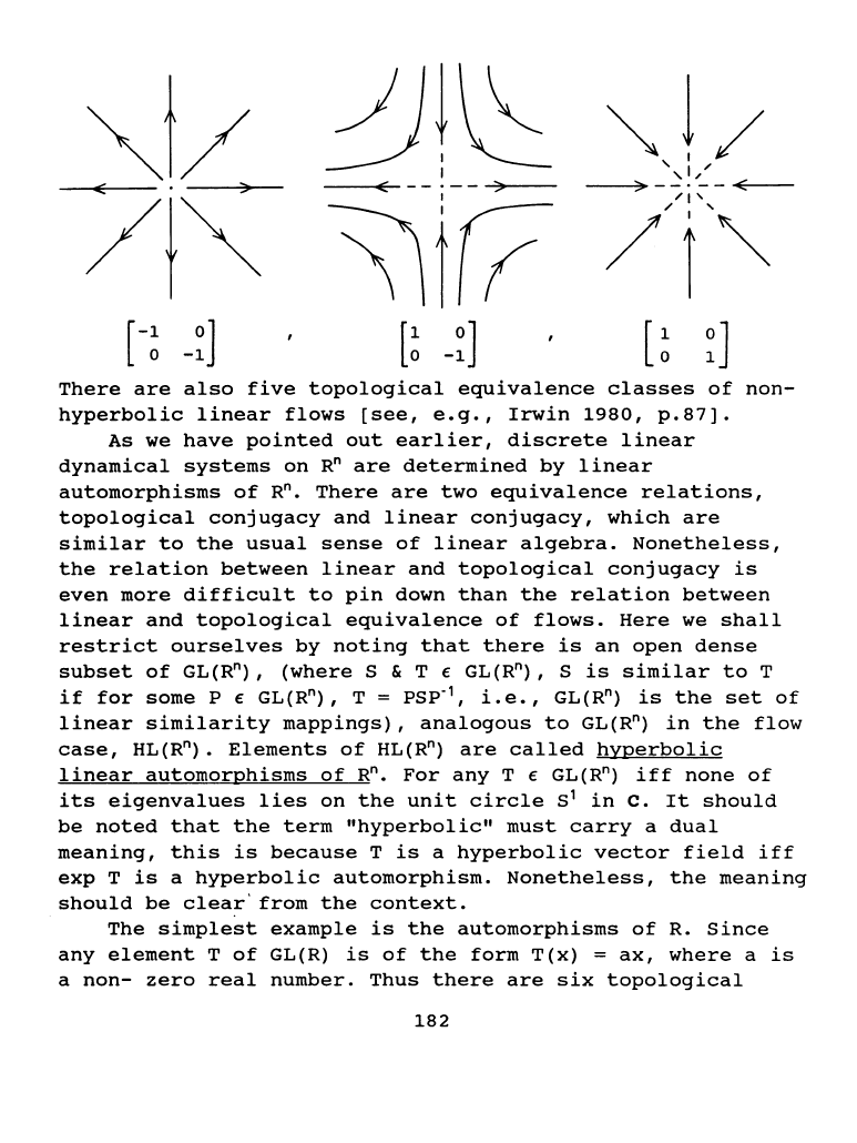
(ii)
Linear
flows
on
R
2
•
The
real
Jordan
form
for
a
real
2x2
matrix
is
one
of
the
following
three
types:
(a)
[
~
~]
,
(b)
!]
(c)
[:
-:
J
where
a,
~.
a,
b £ R
and
b >
o.
One
can
show
that
a
linear
vector
field
on
R
2
is
hyperbolic
iff
(a)
~a
+ o,
(b)
a + o,
(c)
a + o.
181
""'f/
',I/'
~-----~
"I'
/'
t
'""'
[
~
~]
There
are
also
five
topological
equivalence
classes
of
non-
hyperbolic
linear
flows
[see,
e.g.,
Irwin
1980,
p.87].
As
we
have
pointed
out
earlier,
discrete
linear
dynamical
systems
on
R"
are
determined
by
linear
automorphisms
of
R".
There
are
two
equivalence
relations,
topological
conjugacy
and
linear
conjugacy,
which
are
similar
to
the
usual
sense
of
linear
algebra.
Nonetheless,
the
relation
between
linear
and
topological
conjugacy
is
even
more
difficult
to
pin
down
than
the
relation
between
linear
and
topological
equivalence
of
flows.
Here
we
shall
restrict
ourselves
by
noting
that
there
is
an
open
dense
subset
of
GL(R"),
(where
S & T E
GL(R"),
Sis
similar
toT
if
for
some
P E
GL(R"),
T =
psp·l,
i.e.,
GL(R")
is
the
set
of
linear
similarity
mappings),
analogous
to
GL(R")
in
the
flow
case,
HL(R").
Elements
of
HL(R")
are
called
hyperbolic
linear
automorphisms
of
R".
For
any
T E GL(R")
iff
none
of
its
eigenvalues
lies
on
the
unit
circle
s
1
in
c.
It
should
be
noted
that
the
term
"hyperbolic"
must
carry
a
dual
meaning,
this
is
because
T
is
a
hyperbolic
vector
field
iff
exp
T
is
a
hyperbolic
automorphism.
Nonetheless,
the
meaning
should
be
clear'
from
the
context.
The
simplest
example
is
the
automorphisms
of
R.
Since
any
element
T
of
GL(R)
is
of
the
form
T(x)
=
ax,
where
a
is
a
non-
zero
real
number.
Thus
there
are
six
topological
182
conjugacy
classes,
(i)
a <
-1,
(ii)
a =
-1,
(iii)
-1
< a <
o,
(iv)
0 < a <
1,
(v)
a =
1,
(vi)
a >
1.
Clearly,
by
definition,
except
(ii)
and
(v)
are
hyperbolic.
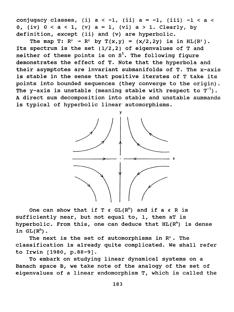
The
map
T:
R'
~
R'
by
T(x,y)
=
(x/2,2y)
is
in
HL(R').
Its
spectrum
is
the
set
(1/2,2}
of
eigenvalues
of
T
and
neither
of
these
points
is
on
s
1
•
The
following
figure
demonstrates
the
effect
of
T.
Note
that
the
hyperbola
and
their
asymptotes
are
invariant
submanifolds
of
T.
The
x-axis
is
stable
in
the
sense
that
positive
iterates
of
T
take
its
points
into
bounded
sequences
(they
converge
to
the
origin).
They-axis
is
unstable
(meaning
stable
with
respect
to
T-
1
).
A
direct
sum
decomposition
into
stable
and
unstable
summands
is
typical
of
hyperbolic
linear
automorphisms.
y
--~~--------
X
One
can
show
that
if
T £ GL(R")
and
if
a e R
is
sufficiently
near,
but
not
equal
to,
1,
then
aT
is
hyperbolic.
From
this,
one
can
deduce
that
HL(R")
is
dense
in
GL(R").
The
next
is
the
set
of
automorphisms
in
R'
•
The
classification
is
already
quite
complicated.
We
shall
refer
to
Irwin
(1980,
p.88-9].
To
embark
on
studying
linear
dynamical
systems
on
a
Banach
space
B,
we
take
note
of
the
analogy
of
the
set
of
eigenvalues
of
a
linear
endomorphism
T,
which
is
called
the
183
