Kurfess T.R. Robotics and Automation Handbook

Подождите немного. Документ загружается.

-20 Robotics and Automation Handbook

−5

−10

0 20 40 60 80 100 120

Human Force (N)

Time (sec)

Z Direction Force

X and Y Direction Force

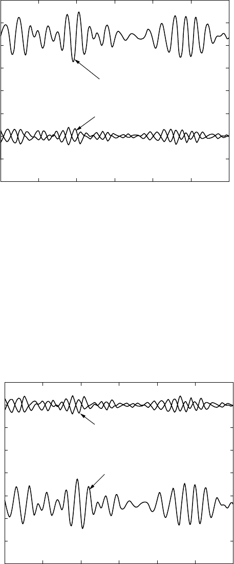
FIGURE 21.16 Human force without compensation.

the operator, after the initial transient, was 11.38 N, approximately 51% of the actual load. In addition,

there are orthogonal disturbances in the X and Y directions due to the rolling, swaying and surging

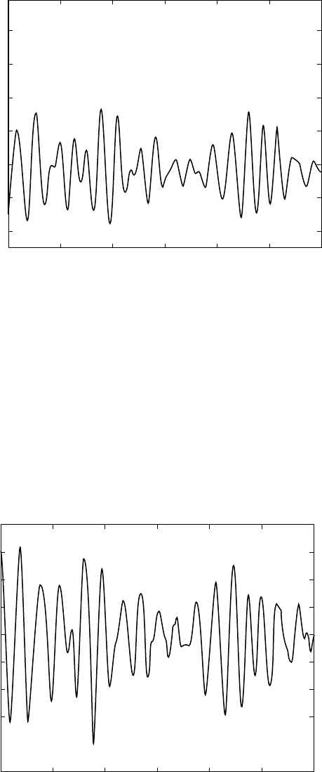
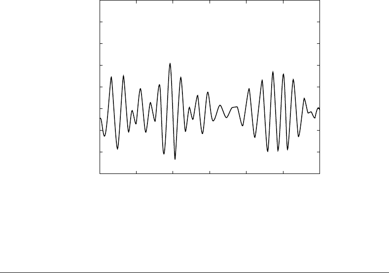
motion of the ship. The resulting tip motion is displayed in Figure 21.17, Figure 21.18, Figure 21.19,

and Figure 21.20. It is clear that the vertical direction is the most sensitive to the sea state. The variation

in the vertical tip position is 22.8 mm. The tracking error above is a function of two inputs: the force

(due to the sea state) applied to the arm and the commanded motion from the force applied by the

operator.

500

−500

−1000

−1500

−3000

−3500

0 20 40 60 80 100 120

Tip Force (N)

Time (sec)

−2000

−2500

Z Direction Force

X and Y Direction Force

FIGURE 21.17 Tip force without compensation.

Robot Simulation 21

-21

1.89

0 20 40 60 80 100 120

X-Direction Tip Position (m)

Time (sec)

1.888

1.886

1.884

1.882

1.88

1.878

1.876

FIGURE 21.18 X tip direction.

The primary motivation for this exercise is to show the potential for robot simulation. In the case above,

studying the control of a robot on the deck of a moving ship could prove quite costly in terms of either

deploying hardware on a ship or designing and constructing a testbed capable of emulating ship motion.

Clearly, the ﬁnal step in the process is validation of the simulation through experimentation. However,

a high ﬁdelity simulation can provide insight into many problems at a fraction of the cost. In addition,

simulation reduces the hazards associated with testing immature control concepts. No one gets hurt if the

simulation fails.

× 10

–3

200 40 60 80 100 120

Y-Direction Tip Position (m)

Time (sec)

−1

−2

−3

−4

−5

FIGURE 21.19 Y tip direction.

-22 Robotics and Automation Handbook

1.22

200 40 60 80 100 120

Z-Direction Tip Position (m)

Time (sec)

1.215

1.21

1.205

1.195

1.19

1.185

1.18

1.2

FIGURE 21.20 Z tip direction.

21.5 Conclusion

This chapter focused on recent developments in robot simulation. The traditional role of robot simulation

in the automotive and aerospace industries still exists but has expanded in terms of its utility and ﬂexi-

bility. However, more advanced engineering tools are providing the ability for rapid prototyping, design

optimization, and hardware in the loop-simulation. With the expanding use of robotics in areas such as

medicine and the battleﬁeld, as well as advancements in haptics and man-machine interfaces, it is likely

that there will be greater interaction between humans and simulation in the near future.

References

Asada, H. and Slotine, J. (1989). Robot Analysis and Control, Wiley Interscience, New York.

Bridges, M. and Diamond, D. (1999). The ﬁnancial impact of teaching surgical residents in the operating

room, Am. J. Surg., Vol. 177, pp. 28–32.

Craig, J. (1989). Introduction to Robotics: Mechanics and Control, 2nd ed., Addison-Wesley, Reading, MA.

Cushieri, A. (1995). Whither minimal access surgery: tribulations and expectations, Am. J. Surg., Vol. 69,

pp. 9–19.

Hawkings, K. and Astle, D. (2001). OpenGL Game Programming, Prima Publishing, Roseville, CA.

Spong, M. and Vidyasagar, M. (1989). Robot Dynamics and Control, John Wiley & Sons, New York.

Van Hoesen, D., Bzorgi, F., Kelsey, A., Wiles, C., and Beeson, K. (1995). Underground radioactive waste

tank remote inspection and sampling, DOE EM Fact Sheet, Gunite and Associated Tanks Operable

Unit at Waste Area Grouping 1 at Oak Ridge National Laboratory, The Department of Energy

Environmental Program.

Woo, M., Neider, J., Davis, T., and Shreiner, D. (1999). OpenGL Programming Guide: The Ofﬁcial Guide to

Learning OpenGL, 3rd ed., Addison-Wesley, Reading, MA.

Yong, Y. and Bonney, M. (1999). Ofﬂine programming, In: Handbook of Industrial Robotics, S. Nof, ed.,

John Wiley & Sons, New York, Chapter 19.

Yoshikawa, T. (1990). Foundations of Robotics: Analysis and Control, MIT Press, Cambridge.

Robot Simulation 21

-23

Appendix A: Matlab Code for The Single DOF Example

syms ai alfai di thi mass g

syms q1 q1_d q1_dd

syms roll pitch yaw heave surge sway

syms roll_d pitch_d yaw_d heave_d surge_d sway_d

syms roll_dd pitch_dd yaw_dd heave_dd surge_dd sway_dd

syms th1 th1d th1dd

syms th2 th2d th2dd

syms th3 th3d th3dd

syms L1 I1x I1y I1z M

pi = sym('pi');

% Symbolically derive motion of base of robot on deck of ship experiencing

% 6 dof of sea motion (roll, pitch, yaw, heave, surge, sway).

R1s=[1 0 0;

0 cos(roll) sin(roll);

0 -sin(roll) cos(roll)];

R2s=[cos(pitch) 0 -sin(pitch);

010;

sin(pitch) 0 cos(pitch)];

R3s=[cos(yaw) sin(yaw) 0;

-sin(yaw) cos(yaw) 0;

0 0 1];

Hsea=[[simple(R1s*R2s*R3s) [surge;sway;heave;]];[0 0 0 1]];

% mask off 3 of 6 sea states (keep sea states in x-z plane)

Hsea=subs(Hsea,'roll',0);

Hsea=subs(Hsea,'yaw',0);

Hsea=subs(Hsea,'sway',0);

% compute kinematics of arm, start off by rotating z from vertical to horizontal

ai=0;alfai=pi/2;di=0;thi=0;

H1=[cos(thi) -sin(thi)*cos(alfai) sin(thi)*sin(alfai) ai*cos(thi);

sin(thi) cos(thi)*cos(alfai) -cos(thi)*sin(alfai) ai*sin(thi);

0 sin(alfai) cos(alfai) di;

0 0 0 1];

ai=L1;alfai=0;di=0;thi=th1;

H2=[cos(thi) -sin(thi)*cos(alfai) sin(thi)*sin(alfai) ai*cos(thi);

sin(thi) cos(thi)*cos(alfai) -cos(thi)*sin(alfai) ai*sin(thi);

0 sin(alfai) cos(alfai) di;

0 0 0 1];

% Homogeneous transform for the robot

H=simple(H1*H2);

% Full homogeneous transform of robot include sea state

H_full=simple(Hsea*H);

% state vector of robot

q=[th1];

% derivitive of state vector

qd=[th1d];

% sea state vector

qs=[pitch;heave;surge];

% sea state velocity

-24 Robotics and Automation Handbook

qsd=[pitch_d;heave_d;surge_d];

% sea state acceleration

qsdd=[pitch_dd;heave_dd;surge_dd];

% velocity computation. Each velocity is velocity of the cg of the line wrt base

coordinate system

% velocity of cg of 2nd link

Ht=simple(Hsea*H1*H2); % homogeneous transform from base to cg of link 2

R2c=Ht((1:3),4); % pull out x, y, z (vector from base to link 2 cg)

V2c=Jacobian(R2c,[q(1);qs])*[qd(1);qsd]; % calculate velocity of cg

of link 2 wrt inertial frame (V = dR/dt = dR/dq * dq/dt)

% rotation matricies from base to each associated coordinate system

R1=transpose(H1(1:3,1:3));

R2=transpose(H2(1:3,1:3));

% angular velocity of each link about cg wrt local coordinate frame

Q1=[0;0;th1d]+[0;0;qsd(1)];

% inertia matrix for each link about center of gravity wrt coordinate frame of

line (same as homogeneous transform, just translated to cg)

I1=[I1x 0 0;0 I1y 0;0 0 I1z];

% Payload information (position/velocity)

Rtip=H_full(1:3,4);

Vtip=Jacobian(Rtip,[q;qs])*[qd;qsd];

% total kinetic energy: T = 1/2 qdot' * I * qdot + 1/2 V' M V

T=1/2*M*(transpose(Vtip)*Vtip)+1/2*transpose(Q1)*I1*Q1;

% potential energy due to gravity

V=M*g*Rtip(3);

%====================================================================

% Energy approach: d/dt(dT/dqd)-dT/dq+dV/dq=Q

% Note: d/dt() = d()/dq * qd + d()/dqd * qdd.

% thus, energy expansion: d(dT/dqd)/dqd * qdd + d(dT/dqd)/dq * qd

-dT/dq + dV/dq = Q.

% first term d(dT/dqd)/dqd is mass matrix, nonlinear terms (coriolis,

centripetal, gravity...)

%====================================================================

% calculate dT/dqdot

dT_qdot=Jacobian(T,qd);

% extract out mass matrix

MassMatrix= simple(Jacobian(dT_qdot,qd));

% now finish off with remaining terms

NLT1=simple(Jacobian(dT_qdot,[q])*[qd]);

NLT2=simple(Jacobian(dT_qdot,transpose(qs))*qsd);

NLT3=simple(Jacobian(dT_qdot,transpose(qsd))*qsdd);

NLT4=simple(transpose(-1*(Jacobian(T,q))));

NLT5=simple(((Jacobian(V,q))));

NLT=simple(NLT1+NLT2+NLT3+NLT4+NLT5);

Appendix B: Matlab Code for The 3-DOF System, Full Sea State

syms ai alfai di thi mass g

syms q1 q1_d q1_dd

syms roll pitch yaw heave surge sway

Robot Simulation 21

-25

syms roll_d pitch_d yaw_d heave_d surge_d sway_d

syms roll_dd pitch_dd yaw_dd heave_dd surge_dd sway_dd

syms th1 th1d th1dd

syms th2 th2d th2dd

syms th3 th3d th3dd

syms L1 L2 L3 L4 L1c L2c L3c L3x L3h L3y L4c

syms I1x I2x I3x I1y I2y I3y I1z I2z I3z

syms m1 m2 m3

pi = sym('pi');

% Symbolically derive motion of base of robot on deck of ship experiencing

% 6 dof of sea motion (roll, pitch, yaw, heave, surge, sway). Use DH

parameters

% to describe this motion in terms of homogeneous transforms.

R1s=[1 0 0;

0 cos(roll) sin(roll);

0 -sin(roll) cos(roll)];

R2s=[cos(pitch) 0 -sin(pitch);

010;

sin(pitch) 0 cos(pitch)];

R3s=[cos(yaw) sin(yaw) 0;

-sin(yaw) cos(yaw) 0;

0 0 1];

Hsea=[[simple(R1s*R2s*R3s) [surge;sway;heave;]];[0 0 0 1]];

ai=-L1;alfai=pi/2;di=0;thi=th1;

H1=[cos(thi) -sin(thi)*cos(alfai) sin(thi)*sin(alfai) ai*cos(thi);

sin(thi) cos(thi)*cos(alfai) -cos(thi)*sin(alfai) ai*sin(thi);

0 sin(alfai) cos(alfai) di;

0 0 0 1];

ai=L2;alfai=0;di=0;thi=th2+pi/2;

H2=[cos(thi) -sin(thi)*cos(alfai) sin(thi)*sin(alfai) ai*cos(thi);

sin(thi) cos(thi)*cos(alfai) -cos(thi)*sin(alfai) ai*sin(thi);

0 sin(alfai) cos(alfai) di;

0 0 0 1];

ai=L2c;alfai=0;di=0;thi=th2+pi/2;

H2c=[cos(thi) -sin(thi)*cos(alfai) sin(thi)*sin(alfai) ai*cos(thi);

sin(thi) cos(thi)*cos(alfai) -cos(thi)*sin(alfai) ai*sin(thi);

0 sin(alfai) cos(alfai) di;

0 0 0 1];

ai=L3x;alfai=0;di=0;thi=th3-pi/2;

H3=[cos(thi) -sin(thi)*cos(alfai) sin(thi)*sin(alfai) ai*cos(thi);

sin(thi) cos(thi)*cos(alfai) -cos(thi)*sin(alfai) ai*sin(thi);

0 sin(alfai) cos(alfai) di;

0 0 0 1];

ai=L3h;alfai=0;di=0;thi=th3-pi/2;

H3h=[cos(thi) -sin(thi)*cos(alfai) sin(thi)*sin(alfai) ai*cos(thi);

sin(thi) cos(thi)*cos(alfai) -cos(thi)*sin(alfai) ai*sin(thi);

0 sin(alfai) cos(alfai) di;

0 0 0 1];

ai=L3c;alfai=0;di=0;thi=th3-pi/2;

H3c=[cos(thi) -sin(thi)*cos(alfai) sin(thi)*sin(alfai) ai*cos(thi);

sin(thi) cos(thi)*cos(alfai) -cos(thi)*sin(alfai) ai*sin(thi);

-26 Robotics and Automation Handbook

0 sin(alfai) cos(alfai) di;

0 0 0 1];

ai=L3y;alfai=0;di=0;thi=pi/2;

H4=[cos(thi) -sin(thi)*cos(alfai) sin(thi)*sin(alfai) ai*cos(thi);

sin(thi) cos(thi)*cos(alfai) -cos(thi)*sin(alfai) ai*sin(thi);

0 sin(alfai) cos(alfai) di;

0 0 0 1];

ai=L4;alfai=-pi/2;di=0;thi=th4-pi/2;

H5=[cos(thi) -sin(thi)*cos(alfai) sin(thi)*sin(alfai) ai*cos(thi);

sin(thi) cos(thi)*cos(alfai) -cos(thi)*sin(alfai) ai*sin(thi);

0 sin(alfai) cos(alfai) di;

0 0 0 1];

H=simple(H1*H2*H3*H4*H5); % Homogeneous transform for the robot

H_full=simple(Hsea*H); % Full homogeneous transform of robot include sea state

q=[th1;th2;th3]; % state vector of robot

qd=[th1d;th2d;th3d]; % derivitive of state vector

qs=[roll;pitch;yaw;heave;surge;sway]; % sea state vector

qsd=[roll_d;pitch_d;yaw_d;heave_d;surge_d;sway_d]; % sea state velocity

qsdd=[roll_dd;pitch_dd;yaw_dd;heave_dd;surge_dd;sway_dd]; % sea

state acceleration

% velocity computation. Each velocity is the velocity of the cg of the line wrt

base coordinate system

% velocity of cg of 2nd link

Ht=simple(Hsea*H1*H2c); % homogeneous transform from base to cg of link 2

R2c=Ht((1:3),4); % pull out x, y, z (vector from base to link 2 cg)

V2c=Jacobian(R2c,[q(1:2);qs])*[qd(1:2);qsd]; % calculate velocity of cg of link 2

wrt inertial frame (V = dR/dt = dR/dq * dq/dt)

% velocity of cg of 3rd link}

Ht=simple(Hsea*H1*H2*H3c);

R3c=Ht((1:3),4);

V3c=simple(Jacobian(R3c,[q;qs])*[qd;qsd]);

% rotation matricies from base to each associated coordinate system

R1=transpose(H1(1:3,1:3));

R2=transpose(H2(1:3,1:3));

R3=transpose(H3(1:3,1:3));

% angular velocity of each link about cg wrt local coordinate frame

Q1=[0;0;th1d]+qsd(1:3);

Q2=simple(R2*R1*Q1+[0;0;th2d]);

Q3=simple([0;0;th3d]+R3*Q2);

% inertia matrix for each link about center of gravity wrt coordinate frame of

line (same as homogeneous transform, translated to cg)

I1=[I1x 0 0;0 I1y 0;0 0 I1z];

I2=[I2x 0 0;0 I2y 0;0 0 I2z];

I3=[I3x 0 0;0 I3y 0;0 0 I3z];

% Payload information (position/velocity)

syms M_payload;

Rtip=H_full(1:3,4);

Vtip=Jacobian(Rtip,[th1;th2;th3;roll;pitch;yaw;heave;surge;sway])*[th1d;th2d;th3d;

roll_d;pitch_d;yaw_d;heave_d;surge_d;sway_d];

Robot Simulation 21

-27

% total kinetic energy: T = 1/2 qdot' * I * qdot + 1/2 V' M V

T=(1/2*transpose(Q1)*I1*Q1 + 1/2*transpose(Q2)*I2*Q2 + 1/2*transpose(Q3)*I3*Q3

+ ... 1/2*m2*transpose(V2c)*V2c + 1/2*m3*transpose(V3c)*V3c) +

1/2*M_payload*(transpose(Vtip)*Vtip);;

% potential energy due to gravity

V=m2*g*R2c(3)+m3*g*R3c(3)+M_payload*g*Rtip(3);

% calculate dT/dqdot

dT_qdot=Jacobian(T,qd);

% extract out mass matrix

MassMatrix= simple(Jacobian(dT_qdot,qd));

% now finish off with remaining terms

NLT1=simple(Jacobian(dT_qdot,[q])*[qd]);

NLT2=simple(Jacobian(dT_qdot,transpose(qs))*qsd);

NLT3=simple(Jacobian(dT_qdot,transpose(qsd))*qsdd);

NLT4=simple(-1*transpose((Jacobian(T,q))));

NLT5=simple(((Jacobian(V,q))));

% translate to C-code

MassMatrix_cc=ccode(MassMatrix);

NLT1_cc=ccode(NLT1);

NLT2_cc=ccode(NLT2);

NLT3_cc=ccode(NLT3);

NLT4_cc=ccode(NLT4);

NLT5_cc=ccode(NLT5);

% calculation of jacobian from tip frame to joint space

LDRDJacobian=simple(Jacobian(H(1:3,4),[th1;th2;th3]));

LDRDJacobian_cc=ccode(LDRDJacobian);

A Survey of

Geometric Vision

Kun Huang

Ohio State University

Yi Ma

University of Illinois

22.1 Introduction

Camera Model and Image Formation

•

3-D Reconstruction

Pipeline

•

Further Readings

22.2 Two-View Geometry

Epipolar Constraint and Essential Matrix

•

Eight-Point Linear

Algorithm

•

Further Readings

22.3 Multiple-View Geometry

Rank Condition on Multiple Views of Point Feature

•

Linear

Reconstruction Algorithm

•

Further Readings

22.4 Utilizing Prior Knowledge of the Scene — Symmetry

Symmetric Multiple-View Rank Condition

•

Reconstruction

from Symmetry

•

Further Readings

22.5 Comprehensive Examples and Experiments

Automatic Landing of Unmanned Aerial Vehicles

•

Automatic

Symmetry Cell Detection, Matching and Reconstruction

•

Semiautomatic Building Mapping and Reconstruction

•

Summary

22.1 Introduction

Vision is one of the most powerful sensing modalities. In robotics, machine vision techniques have been

extensively used in applications such as manufacturing, visual servoing [7, 30], navigation [9, 26, 50, 51],

and robotic mapping [58]. Here the main problem is how to reconstruct both the pose of the camera

and the three-dimensional (3-D) structure of the scene. This reconstruction inevitably requires a good

understanding of the geometry of image formation and 3-D reconstruction. In this chapter, we provide

a survey of the basic theory and some recent advances in the geometric aspects of the reconstruction

problem. Speciﬁcally, we introduce the theory and algorithms for reconstruction from two views (e.g.,

see [29, 31, 33, 40, 67]), multiple views (e.g., see [10, 12, 23, 37, 38, 40]), and a single view (e.g., see

[1, 3, 19, 25, 28, 70, 73, 74]). Since this chapter can only provide a brief introduction to these topics,

the reader is referred to the book [40] for a more comprehensive treatment. Without any knowledge of

the environment, reconstruction of a scene requires multiple images. This is because a single image

is merely a 2-D projection of the 3-D world, for which the depth information is lost. When multiple

images are available from different known viewpoints, the 3-D location of every point in the scene can be

determined uniquely by triangulation (or stereopsis). However, in many applications (especially those for

robot vision), the viewpoints are also unknown. Therefore, we need to recover both the scene structure

-2 Robotics and Automation Handbook

and the camera poses. In computer vision literature, this is referred to as the “structure from motion”

(SFM) problem. To solve this problem, the theory of multiple-view geometry has been developed (e.g., see

[10, 12, 23, 33, 37, 38, 40, 67]). In this chapter, we introduce the basic theory of multiple-view geometry

and show how it can be used to develop algorithms for reconstruction purposes. Speciﬁcally, for the two-

view case, we introduce in Section 22.2 the epipolar constraint and the eight-point structure from motion

algorithm [29, 33, 40]. For the multiple-view case, we introduce in Section 22.3 the rank conditions on

multiple-view matrix [27, 37, 38, 40] and a multiple-view factorization algorithm [37, 40].

Since many robotic applications are performed in a man-made environment such as inside a building

and around an urban area, much of prior knowledge can be exploited for a more efﬁcient and accurate

reconstruction. One kind of prior knowledge that can be utilized is the existence of “regularity” in the

man-made environment. For example, there exist many parallel lines, orthogonal corners, and regular

shapes such as rectangles. In fact, much of the regularity can be captured by the notion of symmetry. It can

be shown that with sufﬁcient symmetry, reconstruction from a single image is feasible and accurate, and

many algorithms have been developed (e.g., see [1, 3, 25, 28, 40, 70, 73]). Interestingly, these symmetry-

based algorithms, in fact, rely on the theory of multiple-view geometry [3, 25, 70]. Therefore, after the

multiple-view case is studied, we introduce in Section 22.4 basic geometry and reconstruction algorithms

associated with imaging and symmetry.

In the remainder of this section, we introduce in Section 22.1.1 basic notation and concepts associated

with image formation that help the development of the theory and algorithms. It is not our intention to

give in this chapter all the details about how the algorithms surveyed can be implemented in real vision

systems. While we will discuss brieﬂy in Section 22.1.1 a pipeline for such a system, we refer the reader to

[40] for all the details.

22.1.1 Camera Model and Image Formation

The camera model we adopt in this chapter is the commonly used pinhole camera model. As shown in

Figure 22.1A, the camera comprises a camera center o and an image plane. The distance from o to the

image plane is the focal length f . For any 3-D point p in the opposite side of the image plane with respect

to o, its image x is obtained by intersecting the line connecting o and p with the image plane. In practice,

it is more convenient to use a mathematically equivalent model by moving the image plane to the “front”

side of the camera center as shown in Figure 22.1B.

There are usually three coordinate frames in our calculation. The ﬁrst one is the world frame, also called

reference frame. The description of any other coordinate frame is the motion between that frame and the

reference frame. The second is the camera frame. The origin of the camera frame is the camera center, and

the z-axis is along the perpendicular line from o to the image plane as shown in Figure 22.1B. The last one

¢

FIGURE 22.1 A: Pinhole imaging model. The image of a point p is the intersecting point x between the image plane

and the ray passing through camera center o. The distance between o and the image plane is f . B: Frontal pinhole

imaging model. The image plane is in front of the camera center o. An image coordinate frame is attached to the image

plane.