Korb K.B., Nicholson A.E. Bayesian Artificial Intelligence

Подождите немного. Документ загружается.

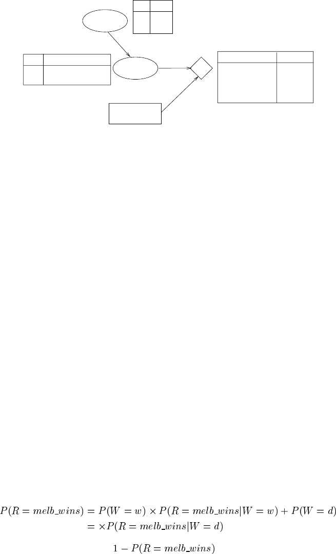
Weather

wet 0.3

dry 0.7

W P(W)

Result

R AB U(R,AB)

melb_wins yes 40

melb_wins no 20

melb_loses no −5

melb_loses yes −20

Accept Bet

wet 0.6

dry 0.25

W P(R=melb_wins|W)

FIGURE 4.3

A decision network for the football team example.

(utility = 20). When her team loses but she didn’t bet, Clare isn’t happy (utility =

-5) but the worst outcome is when she has to buy the dinner wine also (utility = -20).

Clearly, Clare’s preferences reﬂect more than the money at risk. Note also that in

this problem the decision node doesn’t affect any of the variables being modeled,

i.e., there is no explicit outcome variable.

4.3.3 Evaluating decision networks

To evaluate a decision network with a single decision node:

ALGORITHM 4.1

Decision Network Evaluation Algorithm (Single decision)

1. Add any available evidence.

2. For each action value in the decision node:

(a) Set the decision node to that value;

(b) Calculate the posterior probabilities for the parent nodes of the utility

node, as for Bayesian networks, using a standard inference algorithm;

3. Return the action with the highest expected utility.

For the football example, with no evidence, it is easy to see that the expected utility

in each case is the sum of the products of probability and utility for the different

cases. With no evidence added, the probability of Melbourne winning is

and the losing probability is . So the expected utility is:

Note that the probability of the outcomes Clare is interested in (i.e., her team winning

or losing) is independent of the betting decision. With no other information available,

Clare’s decision is to not accept the bet.

4.3.4 Information links

As we mentioned when introducing the types of nodes, there may be arcs from

chance nodes to decision nodes — these are called information links [128, p. 139].

These links are not involved in the basic network evaluation process and have no

associated parameters. Instead, they indicate when a chance node needs to be ob-

served before the decision D is made — but after any decisions prior to D. With an

information link in place, network evaluation can be extended to calculate explic-

itly what decision should be made, given the different values for that chance node.

In other words, a table of optimal actions conditional upon the different relevant

states of affairs can be computed, called a decision table. To calculate the table,

the basic network evaluation algorithm is extended with another loop, as shown in

Algorithm 4.2. We will also refer to this conditional decision table as a policy.

ALGORITHM 4.2

Decision Table Algorithm (Single decision node, with information links)

1. Add any available evidence.

2. For each combination of values of the parents of the decision node:

(a) For each action value in the decision node:

i. Set the decision node to that value;

ii. Calculate the posterior probabilities for the parent nodes of the util-

ity node, as for Bayesian networks, using a standard inference algo-

rithm;

iii. Calculate the resulting expected utility for the action.

(b) Record the action with the highest expected utility in the decision table.

3. Return the decision table.

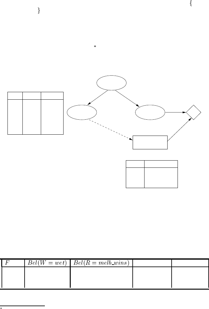
To illustrate the use of information links, suppose that in the football team exam-

ple, Clare was only going to decide whether to accept the bet or not after she heard

the weather forecast. The network can be extended with a Forecast node, represent-

ing the current weather forecast for the match day, which has possible values

sunny,

cloudy or rainy

. Forecast is a child of Weather. There should be an information link

from Forecast to AcceptBet, shown using dashes in Figure 4.4, indicating that Clare

will know the forecast when she makes her decision. Assuming the same CPTs and

utility table, the extended network evaluation computes a decision table, for the de-

cision node given the forecast, also shown in Figure 4.4. Note that most BN software

does not display the expected utilities

. If we want them, we must evaluate the net-

work for each evidence case; these results are given in Table 4.1 (highest expected

utility in each case in bold).

0.60

0.25

0.15

0.40

0.10

0.50

Accept Bet

yes

rainy

sunny

rainy

cloudy

sunny

cloudy

Weather

Information link

W F P(F|W)

dry

wet

Forecast

Result

Accept Bet

Decision Table

cloudy

rainy

sunny

FIGURE 4.4

The football team decision network extended with the Forecast node and an informa-

tion link, with the decision table for AcceptBet computed during network evaluation.

TABLE 4.1

Decisions calculated for football team, given the new evidence node Forecast

EU(AB=yes) EU(AB=no)

rainy 0.720 0.502 10.12 7.55

cloudy 0.211 0.324 -0.56 3.10

sunny 0.114 0.290 -2.61 2.25

GeNIe is one exception that we are aware of.

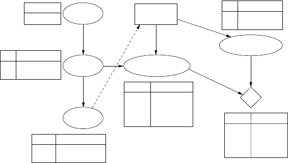
4.3.5 Fever example

Suppose that you know that a fever can be caused by the ﬂu. You can use a ther-

mometer, which is fairly reliable, to test whether or not you have a fever. Suppose

you also know that if you take aspirin it will almost certainly lower a fever to normal.

Some people (about 5% of the population) have a negative reaction to aspirin. You’ll

be happy to get rid of your fever, as long as you don’t suffer an adverse reaction if

you take aspirin. (This is a variation of an example in [128].)

A decision network for this example is shown in Figure 4.5. The Flu node (the

cause) is a parent of the Fever (an effect). That symptom can be measured by a ther-

mometer, whose reading Therm may be somewhat unreliable. The decision is repre-

sented by the decision node Take Aspirin. If the aspirin is taken, it is likely to get rid

of the fever. This change over time is represented by a second node FeverLater.Note

that the aspirin has no effect on the ﬂu and, indeed, that we are not modeling the pos-

sibility that the ﬂu goes away. The adverse reaction to taking aspirin is represented

by Reaction. The utility node, U, shows that the utilities depend on whether or not

the fever is reduced and whether the person has an adverse reaction. The decision

table computed for this network is given in Table 4.2 (highest expected utility in each

case in bold). Note the observing a high temperature changes the decision to taking

the aspirin, but further information about having a reaction reverses that decision.

P(Fe=T|Flu)

0.95

0.02

P(R=T|TA)

0.05

0.00

yes

U(FL,R)

−50

−10

−30

yes

0.05

0.90

0.01

0.02

P(FL|F,TA)

P(Th=T|Fever)

0.90

0.05

P(Flu=T)

0.05

Flu

Reaction

Flu

Fever

Therm

Take

Fever

FeverLater

Aspirin

FIGURE 4.5

A decision network for the fever example.

4.3.6 Types of actions

There are two main types of actions in decision problems, intervening and non-

intervening. Non-intervening actions do not have a direct effect on the chance

variables being modeled, as in Figure 4.6(a). Again, in the football team example,

making a bet doesn’t have any effect on the states of the world being modeled.

TABLE 4.2

Decisions calculated for the fever problem given different values for Therm

and Reaction

Evidence Bel(FeverLater=T) EU(TA=yes) EU(TA=no) Decision

None 0.046 45.27 45.29 no

Therm=F 0.525 45.41 48.41 no

Therm=T 0.273 44.1 19.13 yes

Therm=T & 0.273 -30.32 0 no

Reaction=T

(a) (b)

FIGURE 4.6

Generic decision networks for (a) non-intervening and (b) intervening actions.

Intervening actions do have direct effects on the world, as in Figure 4.6(b). In the

fever example, deciding to take aspirin will affect the later fever situation. Of course

in all decision making, the underlying assumption is that the decision will affect the

utility, either directly or indirectly; otherwise, there would be no decision to make.

The use of the term “intervention” here is apt: since the decision impacts upon the

real world, it is a form of causal intervention as previously discussed in

3.8. Indeed,

one can perform the causal modeling discussed there with the standard Bayesian

network tools by attaching a parent decision node to the chance node that one wishes

to intervene upon. We would prefer these tools to keep decision making and causal

modeling distinct, at least in the human-computer interface. One reason is that causal

intervention is generally (if not necessarily) associated with a single chance node,

whereas the impact of decisions is often more wide-ranging. In any case, the user’s

intent is normally quite different. Decision making is all about optimizing a utility-

driven decision, whereas causal modeling is about explaining and predicting a causal

process under external perturbation.

4.4 Sequential decision making

Thus far, we have considered only single decision problems. Often however a deci-

sion maker has to select a sequence of actions, or a plan.

4.4.1 Test-action combination

A simple example of a sequence of decisions is when the decision maker has the

option of running a test, or more generally making an observation, that will provide

useful information before deciding what further action to take.

In the football decision problem used in the previous section, Clare might have a

choice as to whether to obtain the weather forecast (perhaps by calling the weather

bureau). In the lung cancer example (see

2.2), the physician must decide whether

to order an X-ray, before deciding on a treatment option.

This type of decision problem has two stages:

1. The decision whether to run a test or make an observation

2. The selection of a ﬁnal action

The test/observe decision comes before the action decision. And in many cases,

the test or observation has an associated cost itself, either monetary, or in terms of

discomfort and other physical effects, or both.

A decision network showing the general structure for these test-act decision se-

quences is shown in Figure 4.7. There are now two decision nodes, Test, with values

yes, no ,andAction, with as many values as there are options available. The tempo-

ral ordering of the decisions is represented by a precedence link, shown as a dotted

line.

If the decision is made to run the test, evidence will be obtained for the observa-

tion node Obs, before the Action decision is made; hence there is an information link

from Obs to Action. The question then arises as to the meaning of this information

link if the decision is made not to run the test. This situation is handled by adding an

additional state, unknown,totheObs node and setting the CPT for Obs:

In this generic network, there are arcs from the Action node to both the chance

node X and the utility node U, indicating intervening actions with a direct associated

Precedence link

Information link

Action

Obs

Test

Cost

FIGURE 4.7

Decision network for a test-action sequence of decisions.

cost. However, either of these arcs may be omitted, representing a non-intervening

action or one with no direct cost, respectively.

There is an implicit assumption of no-forgetting in the semantics of a decision

network. The decision maker remembers the past observations and decisions, indi-

cated explicitly by the information and precedence links.

Algorithm 4.3 shows how to use the “Test-Action” decision network for sequential

decision making. We will now look at an decision problem modeled with such a

network and work through the calculations involved in the network evaluation.

ALGORITHM 4.3

Using a “Test-Action” Decision Network

1. Evaluate decision network with any available evidence (other than for the Test

result).

Returns Test decision.

2. Enter Test decision as evidence.

3. If Test decision is ‘yes’

Run test, get result;

Enter test result as evidence to network.

Else

Enter result ‘unknown’ as evidence to network.

4. Evaluate decision network.

Returns Action decision.

4.4.2 Real estate investment example

Paul is thinking about buying a house as an investment. While it looks ﬁne externally,

he knows that there may be structural and other problems with the house that aren’t

immediately obvious. He estimates that there is a 70% chance that the house is really

U(I)

−600

yes

good

bad

good

bad

P(R=good|I,C)

0.95

0.10

0.00

P(R=bad|I,C)

0.05

0.90

0.00

P(R=unk|I,C)

0.00

1.00

good

bad

good

bad

V(BH,C)

5000

−3000

Inspect

Report

yes

P(C=good)

BuyHouse

0.7

Condition

yes

FIGURE 4.8

Decision network for the real estate investment example.

in good condition, with a 30% chance that it could be a real dud. Paul plans to re-

sell the house after doing some renovations. He estimates that if the house really

is in good condition (i.e., structurally sound), he should make a

5,000 proﬁt, but if

it isn’t, he will lose about

3,000 on the investment. Paul knows that he can get a

building surveyor to do a full inspection for

600. He also knows that the inspection

report may not be completely accurate. Paul has to decide whether it is worth it to

have the building inspection done, and then he will decide whether or not to buy the

house.

A decision network for this “test-act” decision problem is shown in Figure 4.8.

Paul has two decisions to make: whether to do have an inspection done and whe-

ther to buy the house. These are represented by the Inspect and BuyHouse decision

nodes, both

yes,no decisions. The condition of the house is represented by the

Condition chance node, with values

good, bad . The outcome of the inspection is

given by node Report, with values

good, bad, unknown . The cost of the inspection

is represented by utility node U, and the proﬁts after renovations (not including the

inspection costs) by a second utility node V. The structure of this network is exactly

that of the general network shown in Figure 4.7.

When Paul decides whether to have an inspection done, he doesn’t have any infor-

mation about the chance nodes, so there are no information links entering the Inspect

decision node. When he decides whether or not to buy, he will know the outcome

of that decision (either a good or bad assessment, or it will be unknown), hence the

information link from Report to BuyHouse. The temporal ordering of his decisions,

ﬁrst about the inspection, and then whether to buy, is represented by the precedence

link from Inspect to BuyHouse. Note that there is a directed path from Inspect to

BuyHouse (via Report) so even if there was no explicit precedence link added by the

knowledge engineer for this problem, the precedence could be inferred from the rest

of the network structure

Given the decision network model for the real-estate investment problem, let’s see

how it can be evaluated to give the expected utilities and hence make decisions.

4.4.3 Evaluation using a decision tree model

In order to show the evaluation of the decision network, we will use a decision tree

representation. The nonleaf nodes in a decision tree are either decision nodes or

chance nodes and the leaves are utility nodes. The nodes are represented using the

same shapes as in decision networks. From each decision node, there is a labeled

link for each alternative decision, and from each chance node, there is a labeled link

for each possible value of that node. A decision tree for the real estate investment

problem is shown in Figure 4.9.

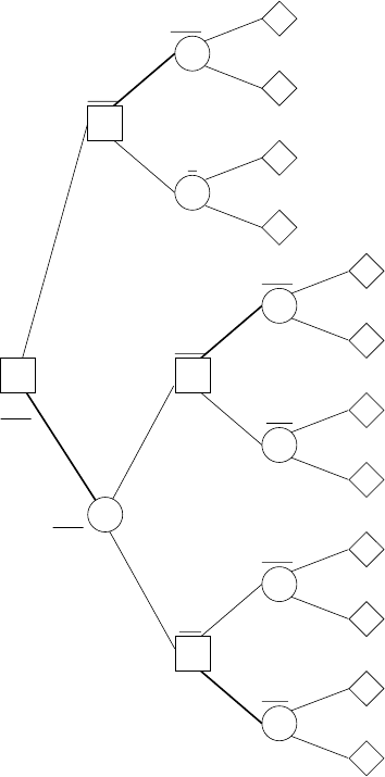
To understand a decision tree, we start with the root node, which in this case is the

ﬁrst decision node, whether or not to inspect the house. Taking a directed path down

the tree, the meaning of the link labels are:

From a decision node, it indicates which decision is made

From a chance node, it indicates which value has been observed

At any point on a path traversal, there is the same assumption of “no-forgetting,”

meaning the decison maker knows all the link labels from the root to the current

position. Each link from a chance node has a probability attached to it, which is the

probability of the variable having that value given the values of all the link labels to

date. That is, it is a conditional probability. Each leaf node has a utility attached to

it, which is the utility given the values of all the link labels on its path from the root.

In our real estate problem, the initial decision is whether to inspect (decision node

I), the result of the inspection report, if undertaken, is represented by chance node R,

the buying decision by BH and the house condition by C. The utilities in the leaves

are combinations of the utilities in the U and V nodes in our decision network. Note

that in order to capture exactly the decision network, we should probably include

the report node in the “Don’t Inspect” branch, but since only the “unknown” branch

would have a non-zero probability, we omit it. Note that there is a lot of redundancy

in this decision tree; the decision network is a much more compact representation.

A decision tree is evaluated as in Algorithm 4.4. Each possible alternative scenario

(of decision and observation combinations) is represented by a path from the root to a

leaf. The utility at that leaf node is the utility that would be obtained if that particular

scenario unfolded. Using the conditional probabilities, expected utilities associated

with the chance nodes can be computed as a sum of products, while the expected

utility for a decision assumes that the action returning the highest expected utility

will be chosen (shown with BOLD, with thicker arcs, in Figure 4.9). These expected

utilities are stored at each non-leaf node in the tree (shown in Figure 4.9 in underlined

italics) as the algorithm works its way recursively back up to the root node.

Some BN software, such as Netica and GeNIe, will add such precedence links automatically.

good

bad

good

bad

good

yes

bad

good

bad

good

4400

−600

4400

−600

0.115

0.885

0.7

bad

good

bad

good

0.3

0.7

0.3

0.695

0.305

0.115

0.885

0.957

0.043

0.957

−3000

5000

2600

2635

0.043

YES

4055

−600

4055

−600

−2682

−3600

FIGURE 4.9

Decision tree evaluation for real estate investment example.