James I.N. Introduction to Circulating Atmospheres
Подождите немного. Документ загружается.

2.3 Numerical weather prediction models
39
Data Coverage
-
AIREP
150*W 120*W 90*W
60"W 30"W
30°E 60*E 90*E I2O"E
I 50'E
i .<>
•.* •
....
.
.. . -
'-~:
m
"
<r
-:
*
•
•
-r •"
^>
l'"
:
1i-k:'-
7-
U
- \, .......
r
•'r-
•\
\
7
{
H
—
>.-'-"•••
'^
si;
v
...
'.
150*W )20*W
90"W
60°W
iO'W
60*t
9O't
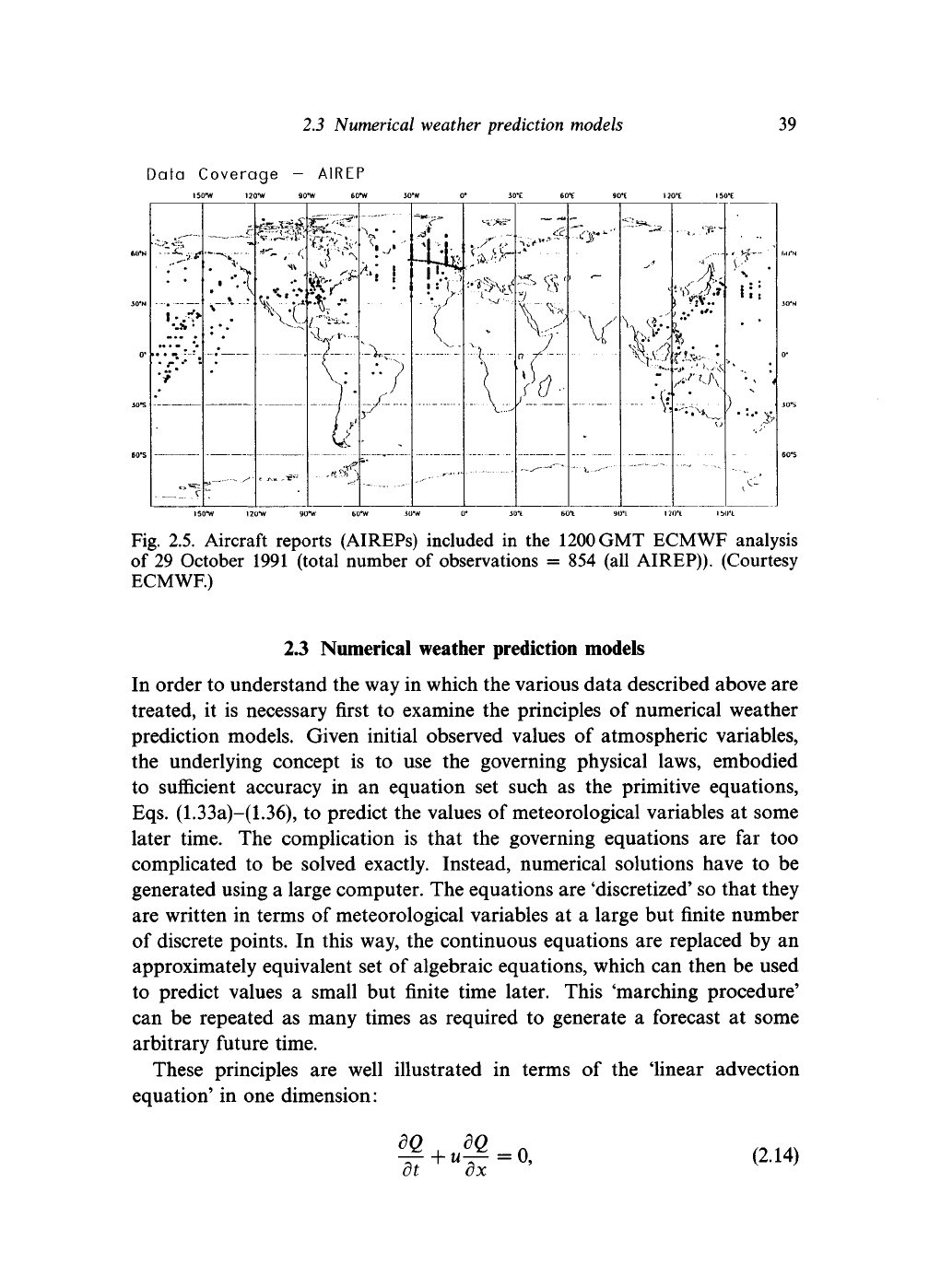
Fig. 2.5. Aircraft reports (AIREPs) included
in
the
1200
GMT ECMWF analysis
of 29 October 1991 (total number
of
observations
=
854 (all AIREP)). (Courtesy
ECMWF.)
2.3 Numerical weather prediction models
In order to understand the way in which the various data described above are
treated,
it is
necessary first
to
examine the principles of numerical weather
prediction models. Given initial observed values
of
atmospheric variables,
the underlying concept
is to
use
the
governing physical laws, embodied
to sufficient accuracy
in an
equation
set
such
as
the primitive equations,
Eqs.
(1.33a)-(1.36), to predict the values of meteorological variables at some
later time. The complication
is
that the governing equations are
far too
complicated
to be
solved exactly. Instead, numerical solutions have
to be
generated using a large computer. The equations are 'discretized' so that they
are written in terms of meteorological variables at
a
large but finite number
of discrete points. In this way, the continuous equations are replaced by an
approximately equivalent set of algebraic equations, which can then be used
to predict values
a
small but finite time later. This 'marching procedure'
can be repeated as many times
as
required
to
generate
a
forecast
at
some
arbitrary future time.
These principles
are
well illustrated
in
terms
of
the linear advection
equation' in one dimension:
(2.14)
40 Observing and modelling global circulations
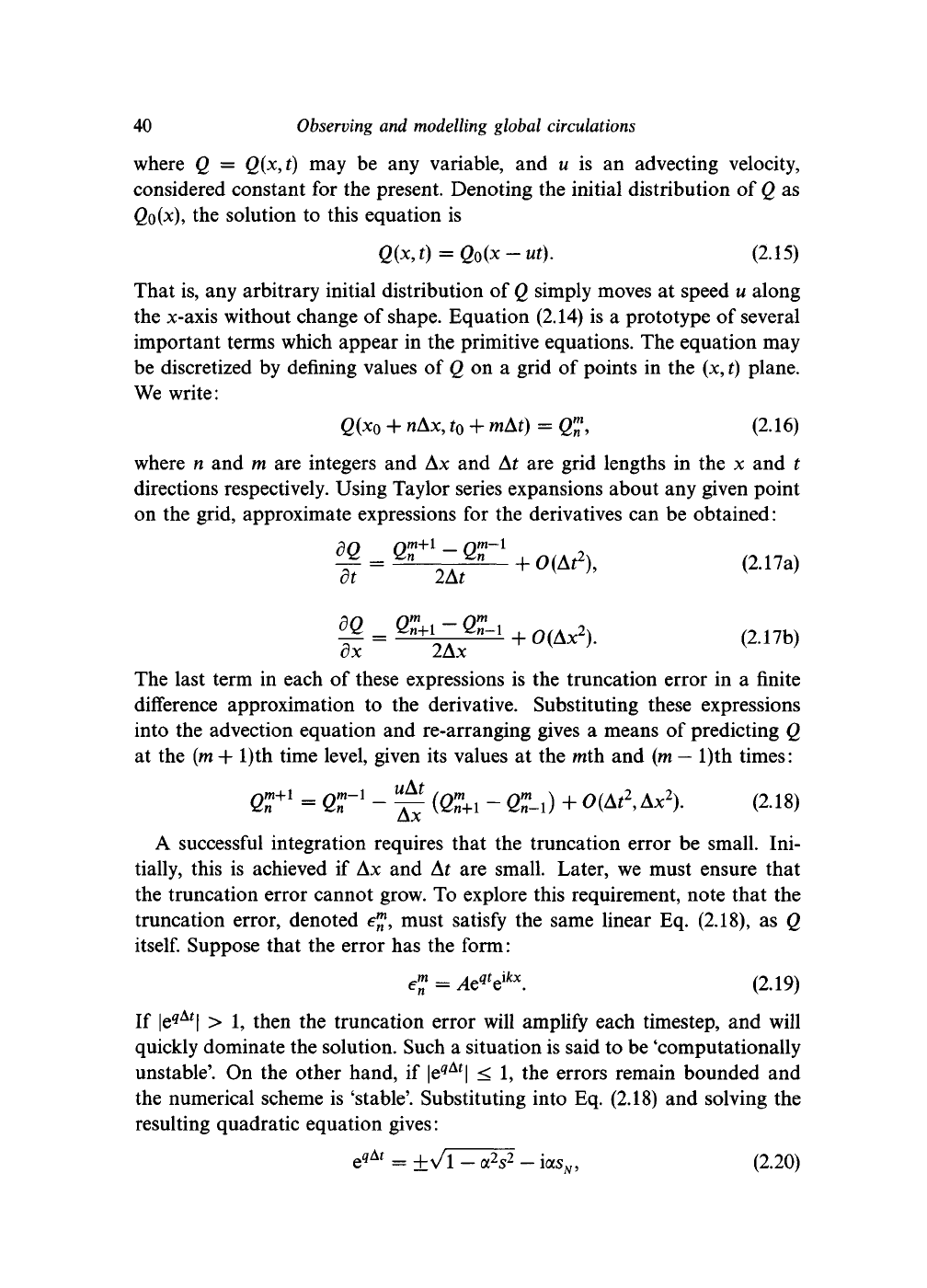
where Q = Q(x,
t)
may be any variable, and u is an advecting velocity,
considered constant for the present. Denoting the initial distribution of
Q
as
Qo(x)
9
the solution to this equation is
Q(x,t)
=
Q
0
(x-ut).
(2.15)
That is, any arbitrary initial distribution of
Q
simply moves at speed u along
the x-axis without change of shape. Equation (2.14) is a prototype of several
important terms which appear in the primitive equations. The equation may
be discretized by defining values of Q on a grid of points in the (x,
t)
plane.
We write:
Q{x
0
+ nAx, t
0
+ mAt) =
Q™,
(2.16)
where n and m are integers and Ax and At are grid lengths in the x and t
directions respectively. Using Taylor series expansions about any given point
on the grid, approximate expressions for the derivatives can be obtained:
8Q
dt 2At
O(At% (2.17a)
(217b)
The last term in each of these expressions is the truncation error in a finite
difference approximation to the derivative. Substituting these expressions
into the advection equation and re-arranging gives a means of predicting Q
at the (m + l)th time level, given its values at the mth and (m
—
l)th times:
^
H )\
A*
2
).
(2.18)
A successful integration requires that the truncation error be small. Ini-
tially, this is achieved if Ax and At are small. Later, we must ensure that
the truncation error cannot grow. To explore this requirement, note that the
truncation error, denoted e^, must satisfy the same linear Eq. (2.18), as Q
itself.
Suppose that the error has the form:
e™
=
Ae
qt
j
kx
.
(2.19)
If
|e^
A
'|
> 1, then the truncation error will amplify each timestep, and will
quickly dominate the solution. Such a situation is said to be 'computationally
unstable'. On the other hand, if
|e^
At
|
< 1, the errors remain bounded and
the numerical scheme is 'stable'. Substituting into Eq. (2.18) and solving the
resulting quadratic equation gives:
= ±Vl - aV - ias
N
, (2.20)

2.3 Numerical weather prediction models 41
where a = uAt/Ax and s
N
= sin(2n/N), NAx = 2n/k being the wavelength of
the error. Stability is ensured if a < 1. If a > 1, errors with some wavelengths
can grow exponentially. This condition for stability, which is usually thought
of as a restriction on the timestep, is called the 'Courant-Friedrich-Lewy'
(CFL) condition:
At < Ax/u for stability. (2.21)
Other finite difference approximations to the advection equation could have
been devised, and these would have had different stability criteria, although
most simple schemes involve some stability condition similar to Eq. (2.21).
This relationship shows that the maximum timestep becomes small as the
grid spacing Ax is reduced. Consequently, any reduction of the truncation by
decreasing Ax means that the timestep has to be reduced to ensure stability.
All these factors combine to mean that the computational effort required
for a numerical solution of the meteorological equations generally rises as a
large power (at least the cube) of the number of grid points.
The CFL condition can be generalized to other, more complicated, equa-
tion sets. The general principle is that 'information' must not travel more
than one grid length in a timestep. Thus, in an equation which describes
wave propagation with phase speed c, a condition for stability is At < Ax/c.
The largest phase speed of waves is often rather large compared to the flow
speeds in the atmosphere, and so this provides a more stringent restriction
on the maximum timestep. For instance, the large flow speeds in the tropo-
sphere are generally less than 100ms"
1
. But the external gravity wave or
'Lamb wave' has a phase speed of around
300
ms"
1
,
and other internal
gravity waves have phase speeds in excess of
100
ms"
1
.
In the early days of
numerical weather prediction, various 'filtered' equation sets were employed
to remove the very fast waves from the system. For instance, equation
sets based on the quasi-geostrophic vorticity equation implicitly include a
thermal wind balance condition which links the wind and temperature fields,
thereby removing gravity waves from the solution. The approach generally
favoured today is to use the primitive equations, which admit gravity wave
solutions, in conjunction with a 'semi-implicit' integration scheme. An impli-
cit integration scheme is one in which data from the unknown (m+ l)th time
level is used in the formulation of the left hand side of the equation. For
example, the linear advection equation may be written:
The spatial derivatives are effectively smoothed in time, and it is easy to
42 Observing and modelling global circulations
show that such a scheme is computationally stable for all At, though its
numerical solutions become increasingly unlike the analytical solutions for
a > 1. Furthermore, obtaining the
Q™
+1
from this finite difference relation
requires the solution of a set of coupled simultaneous equations, one for
each gridpoint. The computational effort for such an implicit scheme is much
greater than the corresponding 'explicit' scheme. In modern semi-implicit
schemes, such a formulation is applied just to those terms in the primitive
equations which generate fast gravity waves; the remainder are handled
explicitly. The limitation on the timestep is then due to the flow speed,
rather than the phase speed of the fastest gravity waves.
Even when At is sufficiently small to guarantee stability, and for the finite
difference approximations to the derivative to be accurate, the numerical
solution to the advection equation can be unrealistic. This is readily seen
if the phase speed of wavelike disturbances, wavelength NAx, is calculated.
The analytic solution reveals that the phase speed should, of
course,
be u for
all wavelengths. But for the finite difference approximation to the equation,
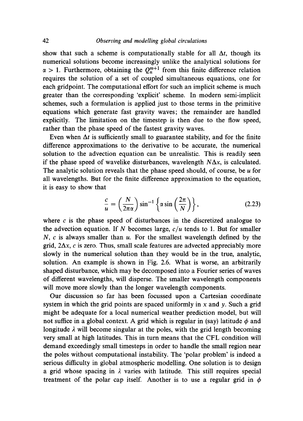
it is easy to show that
H£)H(#)}
where c is the phase speed of disturbances in the discretized analogue to
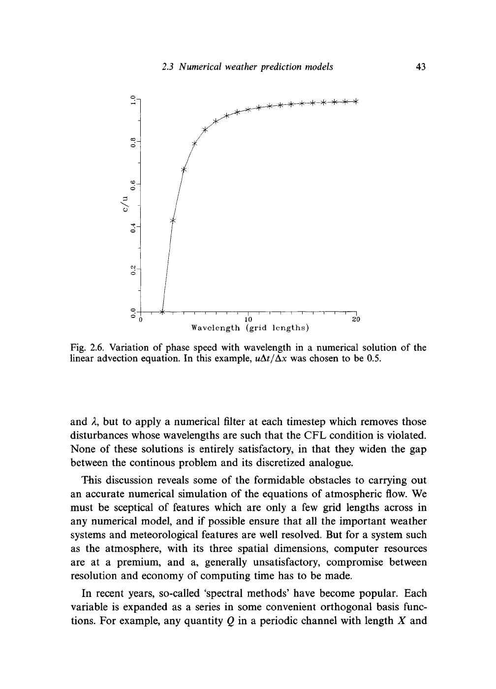
the advection equation. If N becomes large, c/u tends to 1. But for smaller
AT,
c is always smaller than u. For the smallest wavelength defined by the
grid, 2Ax, c is zero. Thus, small scale features are advected appreciably more
slowly in the numerical solution than they would be in the true, analytic,
solution. An example is shown in Fig. 2.6. What is worse, an arbitrarily
shaped disturbance, which may be decomposed into a Fourier series of waves
of different wavelengths, will disperse. The smaller wavelength components
will move more slowly than the longer wavelength components.
Our discussion so far has been focussed upon a Cartesian coordinate
system in which the grid points are spaced uniformly in x and y. Such a grid
might be adequate for a local numerical weather prediction model, but will
not suffice in a global context. A grid which is regular in (say) latitude
</>
and
longitude
X
will become singular at the poles, with the grid length becoming
very small at high latitudes. This in turn means that the CFL condition will
demand exceedingly small timesteps in order to handle the small region near
the poles without computational instability. The 'polar problem' is indeed a
serious difficulty in global atmospheric modelling. One solution is to design
a grid whose spacing in X varies with latitude. This still requires special
treatment of the polar cap
itself.
Another is to use a regular grid in </>
2.3 Numerical weather prediction models
43
10
i
20
Wavelength (grid lengths)
Fig. 2.6. Variation of phase speed with wavelength in
a
numerical solution of the
linear advection equation. In this example, uAt/Ax was chosen to be 0.5.
and
X,
but to apply
a
numerical filter at each timestep which removes those
disturbances whose wavelengths are such that the CFL condition is violated.
None of these solutions is entirely satisfactory, in that they widen the gap
between the continous problem and its discretized analogue.
T4iis discussion reveals some of the formidable obstacles to carrying out
an accurate numerical simulation of the equations of atmospheric
flow.
We
must be sceptical
of
features which are only
a
few grid lengths across
in
any numerical model, and if possible ensure that all the important weather
systems and meteorological features are well resolved. But for a system such
as the atmosphere, with its three spatial dimensions, computer resources
are
at a
premium, and
a,
generally unsatisfactory, compromise between
resolution and economy of computing time has to be made.
In recent years, so-called 'spectral methods' have become popular. Each
variable is expanded as
a
series in some convenient orthogonal basis func-
tions.
For example, any quantity Q in a periodic channel with length
X
and

44 Observing and modelling global circulations
width Y might be represented by a Fourier series:
N M
Q(*,y)
= ZZ
GAM.
sm(nny/YW
2
™* '
x
.
(2.24)
n
=0 m=0
N and M define the wavenumbers at which the series are arbitrarily trun-
cated. Their choice is equivalent to the choice of Ax and Ay in a finite
difference model. Substitution into a linear equation, such as the linear ad-
vection equation, reduces the partial differential equation to a set of ordinary
differential equations. These can be solved accurately by a variety of tech-
niques. Effectively, the method uses all the available information about Q
when computing derivatives, rather than the limited local information used
by a finite difference method. The great advantage of the method is that
the phase speed of wavelike disturbances is represented accurately for all
wavenumbers. Difficulties arise when the governing equations contain non-
linear terms. Terms such as udQ/dx involve multiplying together two Fourier
series,
and, unless the truncation is very severe, the computational labour
involved is very much larger than for the equivalent finite difference scheme.
Spectral methods became competitive with finite difference methods with
the development of the 'spectral transform technique'. In this, each timestep
is divided into two stages:
(i) A gridpoint stage, in which all those products of variables which appear in the
equations are formed.
(ii) A spectral stage. All variables and their required products are represented as
spectral series, and their spatial derivatives are calculated by simple multiplica-
tion. A timestep can then be taken.
The geometry demands rather more complicated basis functions on the
sphere, but the principle remains the same. The appropriate basis functions
are the 'spherical harmonics', which are products of sinusoidal functions rep-
resenting variations in the zonal direction with Legendre functions represent-
ing variations in the meridional direction. Technical details are given in some
references in the bibliography. One very significant advantage of the spectral
transform method on a spherical domain is that it avoids the polar problem
entirely. The spectral representation is isotropic, and resolves features near
the pole in exactly the same detail as features at lower latitudes.
The successful implementation of the method requires a fast transform
between the spectral and gridpoint representations of the variables. The fast
Fourier transform is such a transform suited to periodic domains. Spectral
methods are now at least as popular as finite difference methods for weather
prediction and global circulation models. At reasonably high resolution, the
2.4
The analysis-forecast cycle
45
methods are comparable in computational requirements and are very similar
in accuracy.
This section has concentrated on the 'advective' parts of the solutions
of equations such as the primitive equations. These terms dominate the
solutions for up to the first day or so of a numerical forecast. Beyond this,
the effects of unresolved, subgridscale motions, and of the various heating
and friction processes, become increasingly important. We will concern
ourselves with these topics in Section 2.5.
2.4
The
analysis-forecast cycle
Numerical weather prediction requires initial data defined on some mathemat-
ically specified grid of points covering the Earth's surface. However, observ-
ing stations are not located at mathematically prescribed positions. Rather,
their locations are determined by a succession of historical, geographical and
economical (not to mention military) accidents. What is worse, the observing
stations are not in particularly close proximity over much of the Earth's
surface, and barely serve to resolve the most important weather systems.
The problem of preparing suitable initial data from the heterogeneous, ir-
regular and possibly inadequate set of available observations is known as
'meteorological data analysis' or simply as 'analysis'.
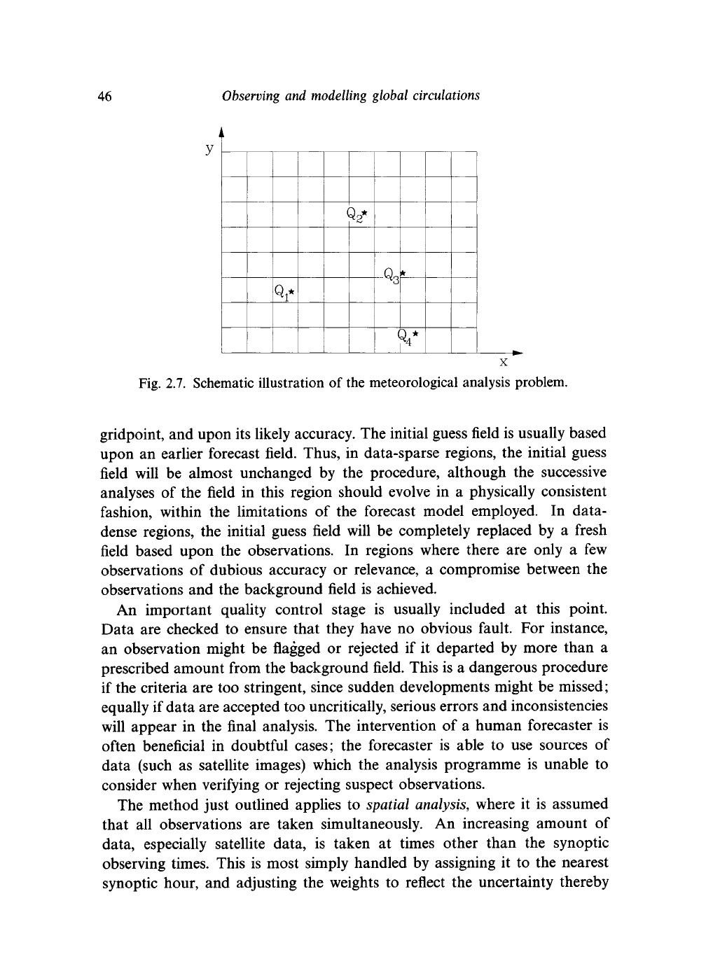
Figure 2.7 shows a schematic view of the problem. The lines represent the
regular grid of data points demanded by a finite difference or spectral model.
The stars represent the actual observations. For simplicity, we assume that
all observations are taken simultaneously, and that we are only dealing with
one level in the atmosphere. If there were many more stars than gridpoints,
our problem would be relatively straightforward. We could simply average
the nearby observations in some way to provide a representative value at
the desired gridpoint. But in practice, the situation is reversed. There are
generally many fewer observations than gridpoints, and in some regions,
there may be virtually no observations.
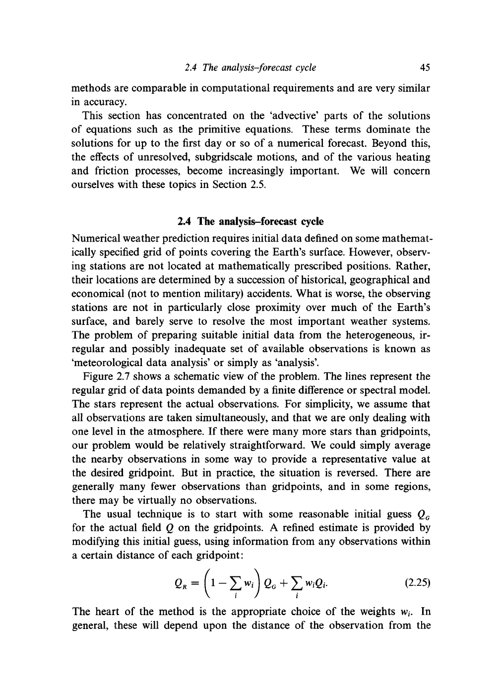
The usual technique is to start with some reasonable initial guess Q
G
for the actual field Q on the gridpoints. A refined estimate is provided by
modifying this initial guess, using information from any observations within
a certain distance of each gridpoint:
The heart of the method is the appropriate choice of the weights w;. In
general, these will depend upon the distance of the observation from the
46
Observing and modelling global circulations
y
(
(
k
X
Fig. 2.7. Schematic illustration of the meteorological analysis problem.
gridpoint, and upon its likely accuracy. The initial guess field is usually based
upon an earlier forecast field. Thus, in data-sparse regions, the initial guess
field will be almost unchanged by the procedure, although the successive
analyses of the field in this region should evolve in a physically consistent
fashion, within the limitations of the forecast model employed. In data-
dense regions, the initial guess field will be completely replaced by a fresh
field based upon the observations. In regions where there are only a few
observations of dubious accuracy or relevance, a compromise between the
observations and the background field is achieved.
An important quality control stage is usually included at this point.
Data are checked to ensure that they have no obvious fault. For instance,
an observation might be flagged or rejected if it departed by more than a
prescribed amount from the background field. This is a dangerous procedure
if the criteria are too stringent, since sudden developments might be missed;
equally if data are accepted too uncritically, serious errors and inconsistencies
will appear in the final analysis. The intervention of a human forecaster is
often beneficial in doubtful cases; the forecaster is able to use sources of
data (such as satellite images) which the analysis programme is unable to
consider when verifying or rejecting suspect observations.
The method just outlined applies to spatial
analysis,
where it is assumed
that all observations are taken simultaneously. An increasing amount of
data, especially satellite data, is taken at times other than the synoptic
observing times. This is most simply handled by assigning it to the nearest
synoptic hour, and adjusting the weights to reflect the uncertainty thereby

2.4
The analysis-forecast cycle
47
introduced. More sophisticated techniques involve inserting such asynoptic
data into the run of a numerical forecast model, modifying the evolving
fields wherever and whenever data becomes available.
Most analysis schemes tend to treat the various meteorological variables
as independent. Thus the wind and temperature analyses are performed
separately. Of course, such fields are not entirely independent. Balance
conditions mean that such variables are related to one another. Thermal wind
balance, linking the wind and temperature fields is an obvious example, as is
gradient wind balance, which relates wind and mass distribution. Similarly,
observations have established that on the larger scale in the extratropics,
the vertical component of vorticity is at least an order of magnitude larger
than the horizontal divergence. This means that the horizontal components
of wind are not entirely independent. In the tropics, other balances are
important, such as a near balance between heating or cooling and ascent or
descent. One goal of more sophisticated schemes is to include such balance
conditions wherever possible.
Nevertheless, at the end of the analysis procedure, the fields are not in
a very good state of dynamical balance. Were the forecast model to be
initialized with these fields, its integration would be dominated by large
amplitude gravity waves of high frequency. Such disturbances are rarely
observed and so an analysed field which gives rise to them in a numerical
integration must be regarded as unphysical. They are removed by including
a process of 'initialization' or balancing between the analysis and forecast
stage. This process involves making rather small adjustments to the fields,
generally considerably smaller than the typical errors of observation. Simple
initialization merely ensures that the horizontal divergence and its rate of
change is set to zero. More sophisticated initialization schemes generate
a pattern of vertical velocity (or divergence) which is consistent with the
observed winds and temperature fields and with the heating rates. In the
midlatitudes, such consistency is related to the quasi-geostrophic approxi-
mation; see Section 1.7. For our purposes in studying the global circulation,
these estimates of the unobservable vertical velocity are extremely useful,
and enable a truly three-dimensional view of atmospheric circulations to be
taken.
A number of the diagnostics to be discussed in this book have been based
on the archived initialized analyses carried out at the European Centre
for Medium Range Weather Forecasts (ECMWF). The ECMWF performs
a global analysis of the atmospheric circulation in the troposphere and
lower stratosphere every six hours. Other centres carry out a comparable
analysis every 12 hours. Once each day, the analysis is integrated forward
48
Observing and modelling global circulations
ooz
Interpolation
cr > p
3-dimensional
analysis
Interpolation
p > cr
Initialization
Forecast
+12 hours
12Z
Interpolation
<r > p
3-dimensional
analysis
Interpolation
p > <r
Initialization
Forecast
+12 hours
OOZ
Interpolation
cr > p
3-dimensional
analysis
Interpolation
p >
<r
Initialization
Forecast
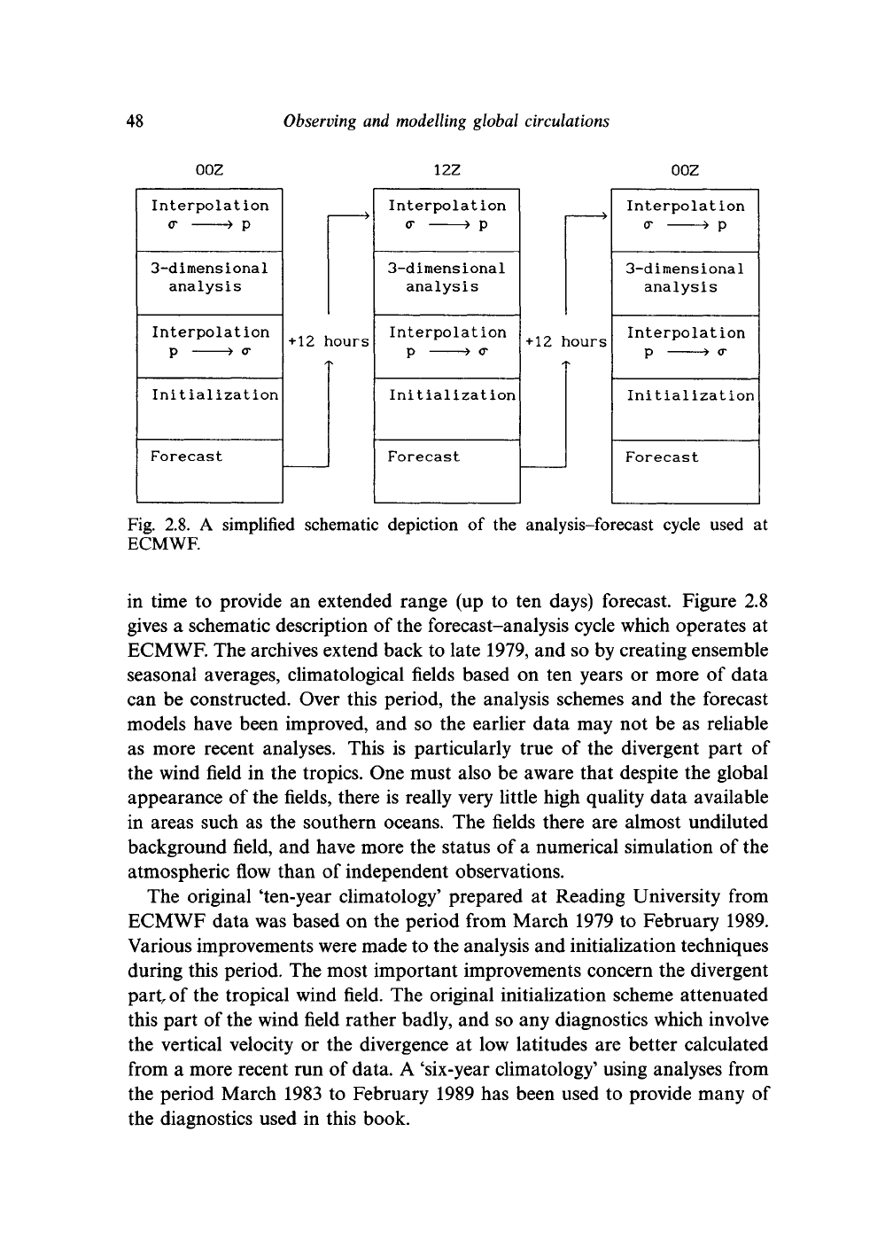
Fig. 2.8. A simplified schematic depiction of the analysis-forecast cycle used at
ECMWF.
in time to provide an extended range (up to ten days) forecast. Figure 2.8
gives a schematic description of the forecast-analysis cycle which operates at
ECMWF. The archives extend back to late 1979, and so by creating ensemble
seasonal averages, climatological fields based on ten years or more of data
can be constructed. Over this period, the analysis schemes and the forecast
models have been improved, and so the earlier data may not be as reliable
as more recent analyses. This is particularly true of the divergent part of
the wind field in the tropics. One must also be aware that despite the global
appearance of the fields, there is really very little high quality data available
in areas such as the southern oceans. The fields there are almost undiluted
background field, and have more the status of a numerical simulation of the
atmospheric flow than of independent observations.
The original 'ten-year climatology' prepared at Reading University from
ECMWF data was based on the period from March 1979 to February 1989.
Various improvements were made to the analysis and initialization techniques
during this period. The most important improvements concern the divergent
part,,
of the tropical wind field. The original initialization scheme attenuated
this part of the wind field rather badly, and so any diagnostics which involve
the vertical velocity or the divergence at low latitudes are better calculated
from a more recent run of data. A 'six-year climatology' using analyses from
the period March 1983 to February 1989 has been used to provide many of
the diagnostics used in this book.
