Jacques J., Raimondo M. Semi-markov risk models for finance, insurance and reliability
Подождите немного. Документ загружается.

248 Chapter 6
In the case of simple annuity the rate can vary only because of time; in the case
of stochastic annuity, clearly it can vary in the same way as the rewards because
the rewards represent the generalization of the payments.
2.2 HSMRWP And Stochastic Annuities Generalization
This section will develop the semi-Markov extension of stochastic annuities.
For the sake of simplification the discrete time case will be discussed before the
continuous one.
As an example of a potential application, it is known that, usually, an insurance
contract makes provision with the premiums paid by the insured person to pay
the claim amounts and to distribute some benefits to the shareholders or to some
public organization. The benefit level but also the premium level could change as
a function of the situation (state) in which the insured person may be.
In our opinion an insurance contract is a typical example of a generalized
stochastic annuity (GSA) as defined below.
Definition 2.1 A generalized stochastic annuity (GSA) is an annuity in which the
payments are a function of the state of the system and the time of the transitions
among the states is stochastic.
The difference between a generalized stochastic annuity and a stochastic annuity,
in discrete time environment, is in the fact that the time of the next transition is a
random variable.
A GSA can be homogeneous or non-homogeneous.
It is homogeneous if the randomness of the time depends only on the duration
between two transitions and it is non-homogeneous if the transitions are functions
of the running time.
The simplest cases, as already shown, can be treated in a homogeneous
environment; in some more composite cases it will require the non-homogeneous
environment
The formulas of a GSA in the homogeneous case are the ones given for the
continuous case in Chapter 4.
Janssen and Manca (2006) give models that could be used to construct a “GSA”
for the insurance problem, using the simple examples given in Haberman and
Pitacco (1999).
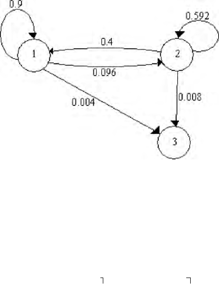
From all these examples we think that the most interesting is the one depicted in
Figure 2.4. in which the weighted directed graph related to the first matrix is
given.
To give an example of a GSA we will develop a case giving four different sets of
data. In the four cases the following two different embedded Markov chains will
be used:
Finance and Insurance models 249
0.9 0.096 0.004
0.4 0.592 0.008
00 1
⎡⎤
⎢⎥
=
⎢⎥
⎢⎥
⎣⎦
P
0.9 0.096 0.004
' 0.8 0.192 0.008 .
00 1
⎡
⎤
⎢
⎥
=
⎢
⎥
⎢
⎥
⎣
⎦
P
(2.7)
For each one of these matrices, we will consider a case without any constraint on
the waiting time distribution functions of the waiting (called
case 1) and another
case with as constraints (called
case 2):
(1) 0.5, , 1, , 3
ij
Fij≥=… . (2.8)
The permanence reward vector will be:
200
1200
0
−
⎡
⎤
⎢
⎥
=
⎢
⎥
⎢
⎥
⎣
⎦
ψ . (2.9)
Figure 2.4
The value
− 200 is the yearly premium that the insured person will pay for
his/her insurance and
1200 is the benefit that she/he will receive from the insurance company when
she/he is disabled.
In the dead state, the permanence reward will be 0.
Using a DTHSMRW model, the following relations are obtained:
()
3
11111
11
2
1
11
() 1 () ( )
() ( ),
t
k
t
k
t
kk
k
Vt H t a b a
beVt
δϑδ
ϑ
δϑ
ϑ
ψ
ϑψ
ϑϑ
==
−
==
=− +
+−
∑∑
∑∑
(2.10)

250 Chapter 6
()
3
22222
11
2
2
11
() 1 () ( )
() ( ),
t
k
t
k
t
kk
k
Vt St a b a
beVt
δϑδ
ϑ
δϑ
ϑ
ψ
ϑψ
ϑϑ
==
−
==
=− +
+−
∑∑
∑∑
(2.11)
3
() 0, 1, ,Vt t T==
… . (2.12)
Our time horizon is ten years and we only consider the due case, as usually
premiums are paid at the beginning of each insured period.
The d.f.
ij
F
, i,j=1,2,3 will be constructed in the program by means of a
pseudorandom number generator taking into account the given constraints; some
of their values are given in
Table 2.1.1 and Table 2.1.2 for the two considered
cases:
Matrix
F
F(1) F(3) F(5)
0.1514 0.144 0.1398 0.3884 0.3767 0.3937 0.5917 0.4724 0.6387
0.0617 0.1675 0.0031 0.3556 0.189 0.1474 0.4568 0.3163 0.3041
1 1 0 1 1 0 1 1 0
F(7) F(9) F(10)
0.744 0.634 0.8232 0.8838 0.8668 0.871 0.9232 0.9384 0.9581
0.6772 0.5729 0.5415 0.855 0.8002 0.8431 0.9527 0.9884 0.9774
1 1 0 1 1 0 1 1 0
Table 2.1.1:case 1
Matrix
F’
F´(1) F´(3) F´(5)
0.5763 0.5712 0.5675 0.7034 0.694 0.6987 0.8125 0.7445 0.8254
0.5273 0.5794 0.4969 0.6801 0.5902 0.57 0.7327 0.654 0.6494
1 1 0 1 1 0 1 1 0
F´(7) F´(9) F´(10)
0.8941 0.8297 0.9207 0.9691 0.9526 0.9455 0.9902 0.9904 0.9905
0.8473 0.7827 0.7698 0.9397 0.8966 0.9226 0.9905 0.991 0.9907
1 1 0 1 1 0 1 1 0
Table 2.1.2: case 2
Table 2.2 presents the results in the four cases (s.s. means starting state).
I Case 1 and matrix P II Case 1 and matrix P´
time s.s. 1 s.s. 2 s.s. 3 s.s. 1 s.s. 2 s.s. 3
1 -200 1200 0 1 -200 1200 0
2 -375 2331 0 2 -375 2298 0
3 -531 3330 0 3 -532 3168 0
4 -664 4234 0 4 -667 3897 0
5 -784 5070 0 5 -791 4532 0
6 -892 5864 0 6 -905 5122 0

Finance and Insurance models 251
7 -973 6584 0 7 -995 5598 0
8 -1045 7215 0 8 -1079 5947 0
9 -1103 7755 0 9 -1151 6167 0
10 -1136 8239 0 10 -1203 6332 0
III Case 2 and matrix P IV Case 2 and matrix P´
s.s. 1 s.s. 2 s.s. 3 s.s. 1 s.s. 2 s.s. 3
1 -200 1200 0 1 -200 1200 0
2 -319 2074 0 2 -319 1787 0
3 -406 2789 0 3 -422 2224 0
4 -473 3419 0 4 -512 2586 0
5 -526 3994 0 5 -595 2900 0
6 -566 4535 0 6 -670 3188 0
7 -587 5023 0 7 -728 3416 0
8 -595 5447 0 8 780 3576 0
9 -591 5804 0 9 -826 3665 0
10 -572 6118 0 10 -860 3726 0
Table 2.2
The reader can easily see that the waiting time d.f. plays a very important role in
the SMP environment and moreover that a consistent change of probabilities in
the embedded Markov chain also gives differences in the results.
The considered constraint on the waiting time d.f gives a sensible decrease of the
waiting time and explains a bigger change in the results.
3 SEMI-MARKOV MODEL FOR INTEREST RATE
STRUCTURE
3.1 The Deterministic Environment
Usually, in a deterministic environment, relation (1.15) implies that:
12
2121
12
11
12
1if ,
(, , )
1if ,
1if .
tt
SttS
tt
SS
tt
ϕ
><
⎧
⎪
====
⎨
⎪
<
>
⎩
(3.1)
This ratio can be seen as a
transformation coefficient giving the value at time
2
t
of a unity account available at time
1
t .
Starting now from (1.14) where
2
S depends on
1
S , we have to suppose that
11 22 11 22
(,)(,) ( ,)( ,)St St kSt kSt k
+
≈⇔ ≈ ∀∈ . (3.2)
Then with
1
1
k
S
= , it results that:

252 Chapter 6
2
11 2 2 1 2
1
(,) (,) (1,) , ,
S
St St t t k
S
+
⎛⎞
≈⇔≈ ∀∈
⎜⎟
⎝⎠
(3.3)
or from the dynamic point of view:
2121 2112
(, , ) (, ,1)SttSSStt
ϕ
ϕ
=⇔=
. (3.4)
This last relation means that it is possible to ignore the third variable and to
simply write:
2112
(, )SSztt
=
. (3.5)
Also taking into account time homogeneity, the transformation coefficient
becomes:
2121 1
() ()S Szt t Szt
=
−= . (3.6)
If 0
t > , then ( ) 1zt > and it results that:
() () 1
rt zt
=
− , (3.7)
and so in this special case, the interest rate
r(t) at time t is defined as in the
classical way.
3.2 The Homogeneous Stochastic Interest Rate Approach
Even with the preceding simplifications, starting with the homogeneity
assumption with respect to time and sums, the interest rate remains one of the
most unpredictable objects.
But as in the case of sums, it is possible to assume that the rate will vary inside a
finite interval:
[
]
', "rrr
∈
. (3.8)
Under the condition (3.8), we start with a model having continuous state space,
but for the sake of applications, as in the previous section, we will work with
only a finite number of states, i.e.:
{
}
12
,, ,
m
rI rr r
∈
= …
. (3.9)
From theoretical and numerical points of view, this assumption implies strong
simplification.
For real life applications, the interest rates are usually fixed in a discrete range,
with as the smallest unit the basic point having for value 0.01%.
As specified above, time will also be on a discrete scale and by means of
DTHSMP of kernel
Q, we will be able to follow the time evolution of the interest
rate in a given time horizon.
The evolution of the interest rate in time gives a yield curve and term structure of
implied forward rates.
This time the functions ( )
ij
F
t represent waiting time d.f. of the interest rate
change from state
i
r to state
j
r , i,j=1,…,m.
Finance and Insurance models 253
The function ( ), ,
ij
tij I
φ
∈ of our semi-Markov process in discrete time process
( , 0,1,..., )
t
Z
Zt T== represents the probability that at time t the interest rate will
be ,
j
r given that the interest rate was
i
r at time 0.
As before, this probability is obtained by the sum of the two terms:
(1 ( ))
ij i
Ht
δ
−
, 1,2,...,ij m
=
, (3.10)
giving the probability of remaining in the starting initial interest rate without any
change in [0,
t] and has meaning only if ij
=
and the second term,
10
() ( )
mt
ih hj
h
bt
θ
θ
φθ
==
−
∑∑
, (3.11)
giving the probability that the interest rate is equal to
j
r after a time t, given that
it was
i
r at time 0 and it reaches the new value with at least one state change (the
first one in
θ
).
If
()
i
θ
Γ
represents the r.v. interest rate related to the period ( 1, ) (0, )T
θ
θ
−
⊂
with values
j
rI∈ and ()
ij
φ
θ
its conditional probability distribution, given that
at time 0 the interest rate was
i
r
, we get the mean interest rate and, as risk
measure, the related variance:
1
(()) ()
m
iijj
j
E
r
θ
φθ
=
Γ=
∑
(3.12)
and:
2
22
11
(()) () () .
mm
iijjijj
jj
rr
σ θ φθ φθ
==
⎛⎞
Γ= −
⎜⎟
⎝⎠
∑∑
(3.13)
3.3 Discount factors
The quantity
()
1
() 1 ()
ii
θθ
−
ϒ=+Γ (3.14)
is the random discount factor related to the period
[
][ ]
1, 0, h
θ
θ
−
⊆ ,
depending on the period and
1
() ().
h
ii
Ah
θ
θ
=
=ϒ
∏
(3.15)
The independence hypothesis among the random discount factors ( )
i
θ
ϒ is
assumed.
This assumption of the independence of stochastic interest rates
i
r
can be
considered equivalent to the independence of the increments of invested sums.
Now the expected values and the variances are given by:

254 Chapter 6
1
1
(()) ()(1 ),
m
iijj
j
Er
θφθ
−
=
ϒ= +
∑
(3.16)
1
() ( ()) ( ()),
h
ii i
hEAh E
θ
ν
θ
=
==ϒ
∏
(3.17)
and for the second ones, generalising the computation of
2
()
X
Y
σ
:
2
221
11
( ( )) ( )(1 ) ( )(1 ) ,
mm
iijjijj
jj
rr
σ θ φθ φθ
−−
==
⎛⎞
ϒ= +− +
⎜⎟
⎝⎠
∑∑
(3.18)
()
2
11
() ,
qq
h
h
iCD
q
Ah S M
θ
θ
σ
⎛⎞
⎜⎟
⎝⎠
==
=
∑∑
(3.19)
where:
()
()
2
1
1
2
1
1
(), ,, ,
(), , , if ,
1if,
q
q
Cir q
r
h
ir h q
D
r
SC
D
h
M
h
θ
θ
θ
θ
σζ ζ ζ
μη η η θ
θ
=
−
−
=
==
⎧
=
<
⎪
=
⎨
⎪
=
⎩
∏
∏
…
…
(3.20)
(, )
q
Ch
θ
∈ C
,
where (, )h
θ
C
is the set of all
θ
−combinations of the set
{
}
1, , h… , and
{}
22
( ) ( ( )),
( ) ( ( )),
1, , .
ii
ii
qq
E
CD h
σ
λσ λ
μλ λ
=ϒ
⎧
⎪
=ϒ
⎨
⎪
=
⎩
∪…
(3.21)
Once the ( )
i
h
γ
are known, it is possible to evaluate the mean present value of a
given financial operation that begins at time 0 and ends at time h.
Clearly, if the value at time 0 is known, the mean value at time h will be obtained
multiplying the initial value by
1()
i
h
ν
.
The knowledge of the expected value and variance of ( )
i
Ah allows important
applications in risk control. In particular it allows decisions and choices in
financial projects by using the mean-variance criterion.
Instead of directly using relation (3.19) for computation, we can use the formula
for the computation of the two independent variables iteratively as follows:
computing first the variance of the first two variables, then considering
successively the result as a variance of one variable and doing the computation of
the variance of two variables, taking the one obtained from the first two and the
third variable and so on.

Finance and Insurance models 255
To illustrate numerically the preceding model, let us suppose that we are
interested in the dynamic evolution of a stochastic interest rate whose possible
values are restricted to the ones given in Table 3.1 and on a ten year time horizon
The first row of the table contains the states and the second row the related
interest rate values.
1 2 3 4 5 6 7 8 9 10 11 12 13 14 15
.03 .035 .04 .045 .05 .055 .06 .065 .07 .075 .08 .085 .09 .095 .1
Table 3.1: homogeneous discount factor states
In this way we have 15 states and 11 time periods, from time period 0 up to the
time period 10.
To get results we constructed a “Mathematica” program able to solve DTHSMP
based on the following data:
a) the transition matrix
P , embedded Markov chain in DTHSMP;
b) the matrix ( )t
F , waiting time distribution functions.
As explained in Chapter 4 the matrix values can be obtained by means of
observation on real data; in this example we filled up both matrices with
pseudorandom numbers.
The transition matrix
P is a square matrix of order 15.
Filling up this matrix we supposed that the transition probabilities were bigger in
the three mean diagonals and that they decrease moving away from them.
The matrix ( )t
F is formed by 11 square matrices, each one of order 15. It results
that:
{
}
{
}
()0,, 1,,15, 1,,10
ij
Ft ij t>∈ ∈……. (3.22)
As we are working in the transient case, with a 10 year horizon time, we consider
all these distribution functions trimmed at the last period.
After the construction of the embedded Markov chain and the distribution
functions we were able to apply the DTHSMP, which is solved as described in
Chapter 4 to get the following probability distributions:
{
}
{
}
,1 ,15
( ), , ( ) with 1, ,15 and 0, ,10
ii
tti t
φ
φ
∈
∈……… (3.23)
to compute for each i, t the interest rate mean values and related standard
deviations.
The results of the example tables are reported on the following pages.
The rows of each table represent the time and the columns the states of the
system at initial time.
The uni-period mean discount factors
(
)
()
i
EV
θ
are reported in Table 3.2, the
mean discount factors form 0 to h, ( ( ))
i
E
Ah in Table 3.3 and the variances
2
(())
i
Ah
σ
in Table 3.4.
3.4 An Applied Example In The Homogeneous Case
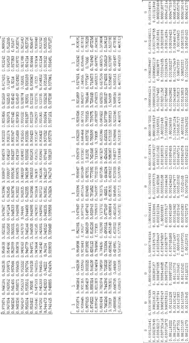
Table 3.2: uniperiod mean discount factors
Table 3.3: mean discount factors
Table 3.4: variance of discount factors
25 6 6 Chapter

Finance and Insurance models 257
3.5 A Factor Discount Example In The Non-Homogeneous
Case
As the interest rate and the discount factors are fundamentally non-homogeneous
phenomena, it is interesting to see that the same kind of example can be provided
also in a non-homogeneous environments.
The state values and their numbers were changed mainly because the number of
results in the non-homogeneous case is by far larger and in this way the results
can be given easily.
All the remarks given in sections 3.2 and 3.3 hold in the non-homogeneous
environment and to repeat all the formulas for this case could be tedious.
This time we have nine states given in
Table 3.5.
States
1 2 3 4 5 6 7 8 9
int rate
0.01 0.015 0.02 0.025 0.03 0.035 0.04 0.045 0.05
disc fact
0.9901 0.9852 0.9804 0.9756 0.9709 0.9662 0.9615 0.9569 0.9524
Table 3.5: discount factor model state
The non-homogeneous uni-period mean discount factors obtained with the
expected value using the transition probabilities ( , )
ij
s
t
φ
, a solution of the
DTNHSMP, are given in
Table 3.6.
The elements in the first column give the couple (s,t) and the corresponding mean
uni-periodic discount factor.
Time
1 2 3 4 5 6 7 8 9
0-1 0.9901 0.9852 0.9804 0.9756 0.9709 0.9662 0.9615 0.9569 0.9524
0-2 0.9887 0.9845 0.9795 0.9755 0.9713 0.9665 0.9619 0.9575 0.9543
0-3 0.9879 0.9828 0.9783 0.9754 0.9712 0.9668 0.9626 0.9584 0.9556
0-4 0.9868 0.9817 0.9773 0.9751 0.9714 0.9673 0.9630 0.9593 0.9570
0-5 0.9856 0.9805 0.9768 0.9751 0.9716 0.9674 0.9637 0.9602 0.9581
0-6 0.9836 0.9791 0.9762 0.9744 0.9715 0.9679 0.9642 0.9615 0.9595
0-7 0.9823 0.9779 0.9756 0.9740 0.9711 0.9685 0.9647 0.9625 0.9614
0-8 0.9806 0.9767 0.9747 0.9735 0.9710 0.9685 0.9658 0.9633 0.9626
0-9 0.9793 0.9759 0.9742 0.9731 0.9709 0.9688 0.9663 0.9647 0.9644
0-10 0.9780 0.9749 0.9737 0.9727 0.9713 0.9693 0.9671 0.9661 0.9662
0-11 0.9760 0.9737 0.9729 0.9720 0.9714 0.9697 0.9687 0.9676 0.9673
3-4 0.9901 0.9852 0.9804 0.9756 0.9709 0.9662 0.9615 0.9569 0.9524
3-5 0.9883 0.9844 0.9798 0.9751 0.9712 0.9669 0.9620 0.9582 0.9552
3-6 0.9866 0.9833 0.9786 0.9745 0.9717 0.9677 0.9624 0.9600 0.9569
3-7 0.9844 0.9819 0.9776 0.9746 0.9716 0.9679 0.9636 0.9615 0.9588
3-8 0.9830 0.9800 0.9764 0.9738 0.9715 0.9682 0.9655 0.9627 0.9600
3-9 0.9809 0.9789 0.9760 0.9731 0.9714 0.9689 0.9662 0.9640 0.9617
3-10 0.9783 0.9775 0.9746 0.9727 0.9711 0.9701 0.9677 0.9650 0.9634
3-11 0.9758 0.9748 0.9739 0.9719 0.9715 0.9704 0.9693 0.9670 0.9659
6-7 0.9901 0.9852 0.9804 0.9756 0.9709 0.9662 0.9615 0.9569 0.9524
6-8 0.9880 0.9833 0.9787 0.9744 0.9705 0.9668 0.9628 0.9592 0.9558
6-9 0.9857 0.9807 0.9766 0.9731 0.9708 0.9673 0.9653 0.9622 0.9588
6-10 0.9822 0.9787 0.9754 0.9734 0.9714 0.9681 0.9662 0.9649 0.9621
6-11 0.9777 0.9754 0.9745 0.9729 0.9715 0.9698 0.9673 0.9669 0.9648
Table 3.6: non-homogeneous uni-period discount factors