Jackson S.L. Research Methods and Statistics: A Critical Thinking Approach

Подождите немного. Документ загружается.

132

■ ■

CHAPTER 5

What if we know an individual’s percentile rank and want to determine

this person’s raw score? Let’s say we know that an individual scored at the

75th percentile on the intelligence test described previously. We want to know

what score has 75% of the scores below it. We begin by using Table A.2 to

determine the z-score for this percentile rank. If the individual is at the 75th

percentile, we know the Area Between Mean and z is .25. How do we know

this? The person scored higher than the 50% of people in the bottom half of

the curve, and .75  .50  .25. Therefore, we look in the column labeled Area

Between Mean and z and find the proportion that is closest to .25. The closest

we come to .25 is .2486, which corresponds to a z-score of 0.67.

Remember, the z-score formula is

z 

X  

______



We know that   100 and   15, and now we know that z  0.67.

What we want to find is the person’s raw score, X. So, let’s solve the equa-

tion for X:

z 

X  

______



z  X  

z    X

Substituting the values we have for , , and z, we find

X  Z  

X  0.67(15)  100

 10.05  100

 110.05

As you can see, the standard normal distribution is useful for determin-

ing how a single score compares with a population or sample of scores and

also for determining probabilities and percentile ranks. Knowing how to use

the proportions under the standard normal curve increases the information

we can derive from a single score.

IN REVIEW Types of Distributions

TYPES OF DISTRIBUTIONS

NORMAL POSITIVELY SKEWED NEGATIVELY SKEWED

Description A symmetrical, A lopsided curve with a A lopsided curve with a

bell- shaped tail extending toward the tail extending toward the

unimodal curve positive or right side negative or left side

z-score transformations applicable? Yes Yes Yes

Percentile ranks and proportions under Yes No No

standard normal curve applicable?

10017_05_ch5_p103-139.indd 132 2/1/08 1:19:10 PM

Data Organization and Descriptive Statistics

■ ■

133

Summary

In this chapter, we discussed data organization and descriptive statistics.

We presented several methods of data organization, including a frequency

distribution, a bar graph, a histogram, and a frequency polygon. We also

discussed the types of data appropriate for each of these methods.

Descriptive statistics that summarize a large data set include measures

of central tendency (mean, median, and mode) and measures of variation

(range, average deviation, and standard deviation). These statistics provide

information about the central tendency or “middleness” of a distribution

of scores and about the spread or width of the distribution, respectively. A

distribution may be normal, positively skewed, or negatively skewed. The

shape of the distribution affects the relationships among the mean, median,

and mode.

CRITICAL

THINKING

CHECK

5.4

1. On one graph, draw two distributions with the same mean but

different standard deviations. Draw a second set of distributions

on another graph with different means but the same standard

deviation.

2. Why is it not possible to use the proportions under the standard

normal curve with skewed distributions?

3. Students in the psychology department at General State University

consume an average of 7 sodas per day with a standard deviation of

2.5. The distribution is normal.

a. What proportion of students consumes an amount equal to or

greater than 6 sodas per day?

b. What proportion of students consumes an amount equal to or

greater than 8.5 sodas per day?

c. What proportion of students consumes an amount between 6 and

8.5 sodas per day?

d. What is the percentile rank for an individual who consumes

5.5 sodas per day?

e. How many sodas would an individual at the 75th percentile

drink per day?

4. Based on what you have learned about z-scores, percentile ranks,

and the area under the standard normal curve, fill in the missing

information in the following table representing performance on an

exam that is normally distributed with



X  55 and S  6.

X z-Score Percentile Rank

John 63

Ray 1.66

Betty 72

10017_05_ch5_p103-139.indd 133 2/1/08 1:19:10 PM

134

■ ■

CHAPTER 5

Finally, we discussed the calculation of z-score transformations as a

means of standardizing raw scores for comparative purposes. Although

z-scores may be used with either normal or skewed distributions, the pro-

portions under the standard normal curve can be applied only to data that

approximate a normal distribution.

Based on our discussion of these descriptive methods, you can begin

to organize and summarize a large data set and also compare the scores of

individuals to the entire sample or population.

frequency distribution

class interval frequency

distribution

qualitative variable

bar graph

quantitative variable

histogram

frequency polygon

descriptive statistics

measure of central tendency

mean

median

mode

measure of variation

range

standard deviation

average deviation

variance

normal curve

normal distribution

kurtosis

mesokurtic

leptokurtic

platykurtic

positively skewed distribution

negatively skewed distribution

z-score (standard score)

standard normal distribution

probability

percentile rank

KEY TERMS

(Answers to odd-numbered exercises appear in

Appendix C.)

1. The following data represent a distribution of

speeds (in miles per hour) at which individuals

were traveling on a highway.

64 80 64 70

76 79 67 72

65 73 68 65

67 65 70 62

67 68 65 64

Organize these data into a frequency distribution

with frequency ( f ) and relative frequency

(rf ) columns.

2. Organize the data in Exercise 1 into a class inter-

val frequency distribution using 10 intervals

with frequency ( f ) and relative frequency (rf )

columns.

3. Which type of figure should be used to represent

the data in Exercise 1—a bar graph, histogram,

or frequency polygon? Why? Draw the appropri-

ate figure for these data.

4. Calculate the mean, median, and mode for the

data set in Exercise 1. Is the distribution nor-

mal or skewed? If it is skewed, what type of

skew is it? Which measure of central tendency

is most appropriate for this distribution, and

why?

5. Calculate the mean, median, and mode for the

following four distributions (a–d):

a b c d

2 1 1 2

2 2 3 3

4 3 3 4

5 4 3 5

8 4 5 6

CHAPTER EXERCISES

10017_05_ch5_p103-139.indd 134 2/1/08 1:19:11 PM

Data Organization and Descriptive Statistics

■ ■

135

a b c d

9 5 5 6

10 5 8 6

11 5 8 7

11 6 8 8

11 6 9 8

8 10

9 11

6. Calculate the range, average deviation, and stand-

ard deviation for the following five distributions:

a. 1, 2, 3, 4, 5, 6, 7, 8, 9

b. 4, 3, 2, 1, 0, 1, 2, 3, 4

c. 10, 20, 30, 40, 50, 60, 70, 80, 90

d. 0.1, 0.2, 0.3, 0.4, 0.5, 0.6, 0.7, 0.8, 0.9

e. 100, 200, 300, 400, 500, 600, 700, 800, 900

7. The results of a recent survey indicate that the

average new car costs $23,000 with a standard

deviation of $3,500. The price of cars is normally

distributed.

a. If someone bought a car for $32,000, what

proportion of cars cost an equal amount or

more than this?

b. If someone bought a car for $16,000, what

proportion of cars cost an equal amount or

more than this?

c. At what percentile rank is a car that sold for

$30,000?

d. At what percentile rank is a car that sold for

$12,000?

e. What proportion of cars were sold for an

amount between $12,000 and $30,000?

f. For what price would a car at the 16th per-

centile have sold?

8. A survey of college students was conducted

during final exam week to assess the number

of cups of coffee consumed each day. The mean

number of cups was 5 with a standard deviation

of 1.5 cups. The distribution was normal.

a. What proportion of students drank 7 or more

cups of coffee per day?

b. What proportion of students drank 2 or more

cups of coffee per day?

c. What proportion of students drank between

2 and 7 cups of coffee per day?

d. How many cups of coffee would an individ-

ual at the 60th percentile rank drink?

e. What is the percentile rank for an individual

who drinks 4 cups of coffee a day?

f. What is the percentile rank for an individual

who drinks 7.5 cups of coffee a day?

9. Fill in the missing information in the following

table representing performance on an exam that

is normally distributed with



X  75 and s  9.

X z-Score Percentile Rank

Ken 73 — —

Drew — 1.55 —

Cecil — — 82

5.1

1. One advantage is that it is easier to “see” the

data set in a graphical representation. A picture

makes it easier to determine where the majority

of the scores are in the distribution. A frequency

distribution requires more reading before a judg-

ment can be made about the shape of the distri-

bution.

2. Gender and type of vehicle driven are qualita-

tive variables, measured on a nominal scale;

thus, a bar graph should be used. The speed at

which the drivers are traveling is a quantitative

variable, measured on a ratio scale. Either a his-

togram or a frequency polygon could be used.

A frequency polygon might be better because of

the continuous nature of the variable.

5.2

1. Because gender and type of vehicle driven are

nominal data, only the mode can be determined;

it is inappropriate to use the median or the mean

with these data. Speed of travel is ratio in scale, so

the mean, median, or mode could be used. Both

the mean and median are better indicators of cen-

tral tendency than the mode. If the distribution is

skewed, however, the mean should not be used.

2. In this case, the mean should not be used

because of the single outlier (extreme score) in

the distribution.

5.3

1. A measure of variation tells us about the spread

of the distribution. In other words, are the scores

CRITICAL THINKING CHECK ANSWERS

10017_05_ch5_p103-139.indd 135 2/1/08 1:19:12 PM

136

■ ■

CHAPTER 5

clustered closely about the mean, or are they

spread over a wide range?

2. The amount of rainfall for the indicated day

is 2 standard deviations above the mean. I

would therefore conclude that the amount of

rainfall was well above average. If the standard

deviation were 2 rather than 0.75, then the

amount of rainfall for the indicated day would

be less than 1 standard deviation above the

mean—above average but not greatly.

5.4

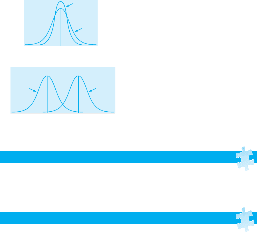
10 30

Same Mean, Different Standard Deviations

Same Standard Deviation, Different Means

Standard

deviation = 2

Standard

deviation = 5

Standard

deviation = 5

Standard

deviation = 5

2. The proportions hold for only normal (sym-

metrical) distributions where one half of the dis-

tribution is equal to the other. If the distribution

were skewed, this condition would be violated.

3. a. .6554

b. .2743

c. .3811

d. 27.43rd

e. 8.68

4. X z-Score Percentile Rank

John 63 1.33 90.82

Ray 45.04 1.66 4.85

Betty 58.48 0.58 72.00

Check your knowledge of the content and key terms

in this chapter with a practice quiz and interactive

flashcards at http://academic.cengage.com/

psychology/jackson, or, for step-by-step practice and

information, check out the Statistics and Research

Methods Workshops at http://academic.cengage

.com/psychology/workshops.

WEB RESOURCES

For hands-on experience using the statistical soft-

ware to conduct the analyses described in this chap-

ter, see Chapters 1 and 2 (“Descriptive Statistics” and

“The z Statistic”) and Exercises 1.1–1.4 and 2.1–2.2

in The Excel Statistics Companion Version 2.0 by

Kenneth M. Rosenberg (Wadsworth, 2007).

STATISTICAL SOFTWARE RESOURCES

10017_05_ch5_p103-139.indd 136 2/1/08 1:19:12 PM

Data Organization and Descriptive Statistics

■ ■

137

CHAPTER 5 SUMMARY AND REVIEW: DATA ORGANIZATION AND DESCRIPTIVE

STATISTICS

This chapter discussed data organization and

descriptive statistics. Several methods of data organi-

zation were presented, including how to design a

frequency distribution, a bar graph, a histogram, and

a frequency polygon. The type of data appropriate for

each of these methods was also discussed.

Descriptive statistics that summarize a large data

set include measures of central tendency (mean,

median, and mode) and measures of variation (range,

average deviation, and standard deviation). These sta-

tistics provide information about the central tendency

or “middleness” of a distribution of scores and about

the spread or width of the distribution, respectively.

A distribution may be normal, positively skewed,

or negatively skewed. The shape of the distribution

affects the relationship among the mean, median, and

mode. Finally, the calculation of z-score transforma-

tions was discussed as a means of standardizing raw

scores for comparative purposes. Although z-scores

can be used with either normal or skewed distribu-

tions, the proportions under the standard normal

curve can only be applied to data that approximate a

normal distribution.

Based on the discussion of these descriptive meth-

ods, you can begin to organize and summarize a large

data set and also compare the scores of individuals to

the entire sample or population.

Chapter 5

■

Study Guide

CHAPTER FIVE REVIEW EXERCISES

(Answers to exercises appear in Appendix C.)

FILL-IN SELF TEST

Answer the following questions. If you have trouble

answering any of the questions, restudy the relevant

material before going on to the multiple-choice self

test.

1. A

is a table in which all of the

scores are listed along with the frequency with

which each occurs.

2. A categorical variable for which each value rep-

resents a discrete category is a

variable.

3. A graphical representation of a frequency dis-

tribution in which vertical bars centered above

scores on the x-axis touch each other to indicate

that the scores on the variable represent related,

increasing values is a

4. Measures of

are numbers

intended to characterize an entire distribution.

5. The

is the middle score in a

distribution after the scores have been arranged

from highest to lowest or lowest to highest.

6. Measures of

are numbers that

indicate how dispersed scores are around the

mean of the distribution.

7. An alternative measure of variation that indicates

the average difference between the scores in a

distribution and the mean of the distribution is

the

8. When we divide the squared deviation scores

by N–1 rather than by N, we are using the

of the population standard

deviation.

9.  represents the

standard

deviation, and S represents the

standard deviation.

10017_05_ch5_p103-139.indd 137 2/1/08 1:19:13 PM

138

■ ■

CHAPTER 5

10. A distribution in which the peak is to the left of

the center point and the tail extends toward the

right is a

skewed distribution.

11. A number that indicates how many standard

deviation units a raw score is from the mean of a

distribution is a .

12. The normal distribution with a mean of 0 and a

standard deviation of 1 is the .

MULTIPLE-CHOICE SELF TEST

Select the single best answer for each of the following

questions. If you have trouble answering any of the

questions, restudy the relevant material.

1. A

is a graphical representation of a

frequency distribution in which vertical bars are

centered above each category along the x-axis

and are separated from each other by a space

indicating that the levels of the variable represent

distinct, unrelated categories.

a. histogram

b. frequency polygon

c. bar graph

d. class interval histogram

2. Qualitative variable is to quantitative variable as

is to .

a. categorical variable; numerical variable

b. numerical variable; categorical variable

c. bar graph; histogram

d. categorical variable and bar graph; numerical

variable and histogram

3. Seven Girl Scouts reported the following indi-

vidual earnings from their sale of cookies: $17,

$23, $13, $15, $12, $19, and $13. In this distribu-

tion of individual earnings, the mean is

the mode and

the median.

a. equal to; equal to

b. greater than; equal to

c. equal to; less than

d. greater than; greater than

4. When Dr. Thomas calculated her students’ his-

tory test scores, she noticed that one student had

an extremely high score. Which measure of cen-

tral tendency should be used in this situation?

a. mean

b. standard deviation

c. median

d. either the mean or the median

5. Imagine that 4,999 people who are penniless live

in Medianville. An individual whose net worth

is $500,000,000 moves to Medianville. Now the

mean net worth in this town is

and the

median net worth is

a. 0; 0

b. $100,000; 0

c. 0; $100,000

d. $100,000; $100,000

6. Middle score in the distribution is to

score occurring with the greatest frequency is to

a. mean; median

b. median; mode

c. mean; mode

d. mode; median

7. Mean is to

as mode is to

a. ordinal, interval, and ratio data only; nominal

data only

b. nominal data only; ordinal data only

c. interval and ratio data only; all types of data

d. none of the above

8. The calculation of the standard deviation differs

from the calculation of the average deviation in

that the deviation scores are:

a. squared.

b. converted to absolute values.

c. squared and converted to absolute values.

d. It does not differ.

9. Imagine that distribution A contains the following

scores: 11, 13, 15, 18, 20. Imagine that distribution

B contains the following scores: 13, 14, 15, 16, 17.

Distribution A has a

standard deviation

and a

average deviation in comparison

to distribution B.

a. larger; larger

b. smaller; smaller

c. larger; smaller

d. smaller; larger

10. Which of the following is not true?

a. All scores in the distribution are used in the

calculation of the range.

10017_05_ch5_p103-139.indd 138 2/1/08 1:19:13 PM

Data Organization and Descriptive Statistics

■ ■

139

b. The average deviation is a more sophisticated

measure of variation than the range, however,

it may not weight extreme scores adequately.

c. The standard deviation is the most sophisti-

cated measure of variation because all scores

in the distribution are used and because it

weights extreme scores adequately.

d. None of the above.

11. If the shape of a frequency distribution is lop-

sided, with a long tail projecting longer to the left

than to the right, how would the distribution be

skewed?

a. normally

b. negatively

c. positively

d. nominally

12. If Jack scored 15 on a test with a mean of 20 and a

standard deviation of 5, what is his z-score?

a. 1.5

b. 1.0

c. 0.0

d. Cannot be determined.

13. Faculty in the physical education department

at State University consume an average of 2,000

calories per day with a standard deviation of

250 calories. The distribution is normal. What

proportion of faculty consumes an amount

between 1,600 and 2,400 calories?

a. .4452

b. .8904

c. .50

d. None of the above

14. If the average weight for women is normally

distributed with a mean of 135 pounds and a

standard deviation of 15 pounds, then approxi-

mately 68% of all women should weigh between

and

pounds.

a. 120; 150

b. 120; 135

c. 105; 165

d. Cannot say from the information given.

15. Sue’s first philosophy exam score is 1 standard

deviation from the mean in a normal distribution.

The test has a mean of 82 and a standard devia-

tion of 4. Sue’s percentile rank would be approxi-

mately:

a. 78%.

b. 84%.

c. 16%.

d. Cannot say from the information given.

SELF TEST PROBLEMS

1. Calculate the mean, median, and mode for the

following distribution.

1, 1, 2, 2, 4, 5, 8, 9, 10, 11, 11, 11

2. Calculate the range, average deviation, and stand-

ard deviation for the following distribution.

2, 2, 3, 4, 5, 6, 7, 8, 8

3. The results of a recent survey indicate that the

average new home costs $100,000 with a standard

deviation of $15,000. The price of homes is nor-

mally distributed.

a. If someone bought a home for $75,000, what

proportion of homes cost an equal amount or

more than this?

b. At what percentile rank is a home that sold for

$112,000?

c. For what price would a home at the 20th per-

centile have sold?

10017_05_ch5_p103-139.indd 139 2/1/08 1:19:14 PM

140

Correlational Methods and

Statistics

CHAPTER

Conducting Correlational Research

Magnitude, Scatterplots, and Types of Relationships

Magnitude

Scatterplots

Positive Relationships

Negative Relationships

No Relationship

Curvilinear Relationships

Misinterpreting Correlations

The Assumptions of Causality and Directionality

The Third-Variable Problem

Restrictive Range

Curvilinear Relationships

Prediction and Correlation

Statistical Analysis: Correlation Coefficients

Pearson’s Product-Moment Correlation Coefficient: What It Is and What It Does

Calculations for the Pearson Product-Moment Correlation • Interpreting the Pearson

Product-Moment Correlation

Alternative Correlation Coefficients

Advanced Correlational Techniques: Regression Analysis

Summary

10017_06_ch6_p140-162.indd 140 2/1/08 1:22:43 PM

Correlational Methods and Statistics

■ ■

141

Learning Objectives

• Describe the differences among strong, moderate, and weak correlation

coefficients.

• Draw and interpret scatterplots.

• Explain negative, positive, curvilinear and no relationship between

variables.

• Explain how assuming causality and directionality, the third-variable

problem, restrictive ranges, and curvilinear relationships can be prob-

lematic when interpreting correlation coefficients.

• Explain how correlations allow us to make predictions.

• Describe when it would be appropriate to use the Pearson product-

moment correlation coefficient, the Spearman rank-order correla-

tion coefficient, the point-biserial correlation coefficient, and the phi

coefficient.

• Calculate the Pearson product-moment correlation coefficient for two

variables.

• Determine and explain r

for a correlation coefficient.

• Explain regression analysis.

• Determine the regression line for two variables.

n this chapter, we will discuss correlational research methods and cor-

relational statistics. As a research method, correlational designs allow

you to describe the relationship between two measured variables. A

correlation coefficient (descriptive statistic) helps by assigning a numeri-

cal value to the observed relationship. We will begin with a discussion of

how to conduct correlational research, the magnitude and the direction of

correlations, and graphical representations of correlations. We will then

turn to special considerations when interpreting correlations, how to use

correlations for predictive purposes, and how to calculate correlation coef-

ficients. Last, we will discuss an advanced correlational technique, regres-

sion analysis.

Conducting Correlational Research

When conducting correlational studies, researchers determine whether two

variables (for example, height and weight, or smoking and cancer) are related

to each other. Such studies assess whether the variables are “correlated” in

some way: Do people who are taller tend to weigh more, or do those who

smoke tend to have a higher incidence of cancer? As we saw in Chapter 1,

the correlational method is a type of nonexperimental method that describes

the relationship between two measured variables. In addition to describing

a relationship, correlations allow us to make predictions from one variable

to another. If two variables are correlated, we can predict from one variable

to the other with a certain degree of accuracy. For example, knowing that

10017_06_ch6_p140-162.indd 141 2/1/08 1:22:44 PM