Jackson S.L. Research Methods and Statistics: A Critical Thinking Approach
Подождите немного. Документ загружается.

122
■ ■
CHAPTER 5
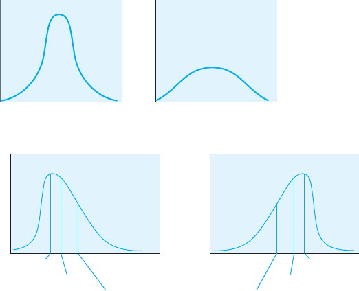
curve on the right side of Figure 5.5. This is a platykurtic curve—platy means
broad or flat. Platykurtic curves are short and more dispersed (broader). In
a platykurtic curve, there are many scores around the middle score that all
have a similar frequency.
Positively Skewed Distributions. Most distributions do not approximate
a normal or bell-shaped curve. Instead they are skewed, or lopsided. In a
skewed distribution, scores tend to cluster at one end or the other of the
x-axis, with the tail of the distribution extending in the opposite direction.
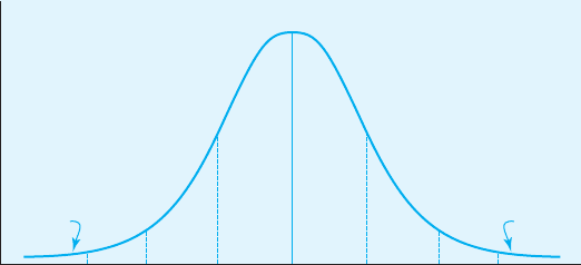
In a positively skewed distribution, the peak is to the left of the center
point, and the tail extends toward the right, or in the positive direction
(see Figure 5.6).
Notice that what skews the distribution, or throws it off center, are the
scores toward the right, or positive direction. A few individuals have extremely
high scores that pull the distribution in that direction. Notice also what this
does to the mean, median, and mode. These three measures do not have the
same value, nor are they all located at the center of the distribution as they are
in a normal distribution. The mode—the score with the highest frequency—is
the high point on the distribution. The median divides the distribution in half.
The mean is pulled in the direction of the tail of the distribution; that is, the
few extreme scores pull the mean toward them and inflate it.
Negatively Skewed Distributions. The opposite of a positively skewed
distribution is a negatively skewed distribution—a distribution in which
the peak is to the right of the center point, and the tail extends toward the
left, or in the negative direction. The term negative refers to the direction of
platykurtic Normal curves
that are short and more
dispersed (broader).
platykurtic Normal curves
that are short and more
dispersed (broader).
positively skewed
distribution A distribution
in which the peak is to the left
of the center point, and the tail
extends toward the right, or in
the positive direction.
positively skewed
distribution A distribution
in which the peak is to the left
of the center point, and the tail
extends toward the right, or in
the positive direction.
negatively skewed
distribution A distribution
in which the peak is to the right
of the center point, and the tail
extends toward the left, or in the
negative direction.
negatively skewed
distribution A distribution
in which the peak is to the right
of the center point, and the tail
extends toward the left, or in the
negative direction.
FIGURE 5.5
Types of
distributions:
leptokurtic and
platykurtic
Leptokurtic Platykurtic
FIGURE 5.6
Positively and
negatively skewed
distributions
Negatively Skewed DistributionPositively Skewed Distribution
Mode
Median
Mean
Mode
Median
Mean
10017_05_ch5_p103-139.indd 122 2/1/08 1:19:04 PM
Data Organization and Descriptive Statistics
■ ■
123
the skew. As can be seen in Figure 5.6, in a negatively skewed distribution,
the mean is pulled toward the left by the few extremely low scores in the dis-
tribution. As in all distributions, the median divides the distribution in half,
and the mode is the most frequently occurring score in the distribution.
Knowing the shape of a distribution provides valuable information about
the distribution. For example, would you prefer to have a negatively skewed
or positively skewed distribution of exam scores for an exam that you have
taken? Students frequently answer that they would prefer a positively
skewed distribution because they think the term positive means good. Keep
in mind, though, that positive and negative describe the skew of the distribu-
tion, not whether the distribution is “good” or “bad.” Assuming that the
exam scores span the entire possible range (say, 0–100), you should prefer a
negatively skewed distribution—meaning that most people have high scores
and only a few have low scores.
Another example of the value of knowing the shape of a distribution
is provided by Harvard paleontologist Stephen Jay Gould (1985). Gould
was diagnosed in 1982 with a rare form of cancer. He immediately began
researching the disease and learned that it was incurable and had a median
mortality rate of only 8 months after discovery. Rather than immediately
assuming that he would be dead in 8 months, Gould realized this meant
that half of the patients lived longer than 8 months. Because he was diag-
nosed with the disease in its early stages and was receiving high-quality
medical treatment, he reasoned that he could expect to be in the half of the
distribution that lived beyond 8 months. The other piece of information that
Gould found encouraging was the shape of the distribution. Look again at
the two distributions in Figure 5.6, and decide which you would prefer in
this situation. With a positively skewed distribution, the cases to the right
of the median could stretch out for years; this is not true for a negatively
skewed distribution. The distribution of life expectancy for Gould’s disease
was positively skewed, and Gould was obviously in the far right-hand tail
of the distribution because he lived and remained professionally active for
another 20 years.
z-Scores
The descriptive statistics and types of distributions discussed so far are
valuable for describing a sample or group of scores. Sometimes, however,
we want information about a single score. For example, in our exam score
distribution, we may want to know how one person’s exam score compares
with those of others in the class. Or we may want to know how an indi-
vidual’s exam score in one class, say psychology, compares with the same
person’s exam score in another class, say English. Because the two distribu-
tions of exam scores are different (different means and standard deviations),
simply comparing the raw scores on the two exams does not provide this
information. Let’s say an individual who was in the psychology exam dis-
tribution used as an example earlier in the chapter scored 86 on the exam.
Remember, the exam had a mean of 74.00 with a standard deviation (S) of
13.64. Assume that the same person took an English exam and made a score
10017_05_ch5_p103-139.indd 123 2/1/08 1:19:05 PM

124
■ ■
CHAPTER 5
of 91, and that the English exam had a mean of 85 with a standard devia-
tion of 9.58. On which exam did the student do better? Most people would
immediately say the English exam because the score on this exam was
higher. However, we are interested in how well this student did in compari-
son to everyone else who took the exams. In other words, how well did the
individual do in comparison to those taking the psychology exam versus in
comparison to those taking the English exam?
To answer this question, we need to convert the exam scores to a form we
can use to make comparisons. A z-score or standard score is a measure of how
many standard deviation units an individual raw score falls from the mean of
the distribution. We can convert each exam score to a z-score and then compare
the z-scores because they will be in the same unit of measurement. You can
think of z-scores as a translation of raw scores into scores of the same language
for comparative purposes. The formulas for a z-score transformation are
z
X
X
______
S
and
z
X
______
where z is the symbol for the standard score. The difference between the two
formulas is that the first is used when calculating a z-score for an individual
in comparison to a sample, and the second is used when calculating a z-score
for an individual in comparison to a population. Notice that the two formu-
las do exactly the same thing—indicate the number of standard deviations
an individual score is from the mean of the distribution.
Conversion to a z-score is a statistical technique that is appropriate for
use with data on an interval or ratio scale of measurement (scales for which
means are calculated). Let’s use the formula to calculate the z-scores for the
previously mentioned student’s psychology and English exam scores. The
necessary information is summarized in Table 5.11.
To calculate the z-score for the English test, we first calculate the dif-
ference between the score and the mean, and then divide by the standard
deviation. We use the same process to calculate the z-score for the psychol-
ogy exam. These calculations are as follows:
z
English
X
X
______
S
91 85
_______
9.58
6
____
9.58
0.626
z
psychology
X
X
______
S
86 74
_______
13.64
12
_____
13.64
0.880
z-score (standard score)
A number that indicates how
many standard deviation units a
raw score is from the mean of a
distribution.
z-score (standard score)
A number that indicates how
many standard deviation units a
raw score is from the mean of a
distribution.
TABLE 5.11 Raw Score (X), Sample Mean (
X ), and Standard
Deviation (S) for English and Psychology Exams
X
X S
English 91 85 9.58
Psychology 86 74 13.64
10017_05_ch5_p103-139.indd 124 2/1/08 1:19:06 PM
Data Organization and Descriptive Statistics
■ ■
125
The individual’s z-score for the English test is 0.626 standard deviation
above the mean, and the z-score for the psychology test is 0.880 standard
deviation above the mean. Thus, even though the student answered more
questions correctly on the English exam (had a higher raw score) than on
the psychology exam, the student performed better on the psychology exam
relative to other students in the psychology class than on the English exam
in comparison to other students in the English class.
The z-scores calculated in the previous example were both positive,
indicating that the individual’s scores were above the mean in both distri-
butions. When a score is below the mean, the z-score is negative, indicating
that the individual’s score is lower than the mean of the distribution. Let’s
go over another example so that you can practice calculating both positive
and negative z-scores.
Suppose you administered a test to a large sample of people and com-
puted the mean and standard deviation of the raw scores, with the following
results:
X 45
S 4
Suppose also that four of the individuals who took the test had the following
scores:
Person Score (X)
Rich 49
Debbie 45
Pam 41
Henry 39
Let’s calculate the z-score equivalents for the raw scores of these
individuals, beginning with Rich:
z
Rich
X
Rich
X
________
S
49 45
_______
4
4
__
4
1
Notice that we substitute Rich’s score (X
Rich
) and then use the group mean
(
X ) and the group standard deviation (S). The positive sign () indicates that
the z-score is positive, or above the mean. We find that Rich’s score of 49 is
1 standard deviation above the group mean of 45.
Now let’s calculate Debbie’s z-score:
z
Debbie
X
Debbie
X
__________
S
45 45
_______
4
0
__
4
0
Debbie’s score is the same as the mean of the distribution. Therefore, her
z-score is 0, indicating that she scored neither above nor below the mean. Keep
in mind that a z-score of 0 does not indicate a low score—it indicates a score
right at the mean or average. See if you can calculate the z-scores for Pam and
Henry on your own. Do you get z
Pam
1 and z
Henry
1.5? Good work!
In summary, the z-score tells whether an individual raw score is above
the mean (a positive z-score) or below the mean (a negative z-score), and
10017_05_ch5_p103-139.indd 125 2/1/08 1:19:06 PM
126
■ ■
CHAPTER 5
it tells how many standard deviations the raw score is above or below the
mean. Thus, z-scores are a way of transforming raw scores to standard scores
for purposes of comparison in both normal and skewed distributions.
z-Scores, the Standard Normal Distribution,
Probability, and Percentile Ranks
If the distribution of scores for which you are calculating transformations
(z-scores) is normal (symmetrical and unimodal), then it is referred to as
the standard normal distribution—a normal distribution with a mean of 0
and a standard deviation of 1. The standard normal distribution is actually
a theoretical distribution defined by a specific mathematical formula. All
other normal curves approximate the standard normal curve to a greater
or lesser extent. The value of the standard normal curve is that it provides
information about the proportion of scores that are higher or lower than any
other score in the distribution. A researcher can also determine the prob-
ability of occurrence of a score that is higher or lower than any other score
in the distribution. The proportions under the standard normal curve hold
for only normal distributions—not for skewed distributions. Even though
z-scores may be calculated on skewed distributions, the proportions under
the standard normal curve do not hold for skewed distributions.
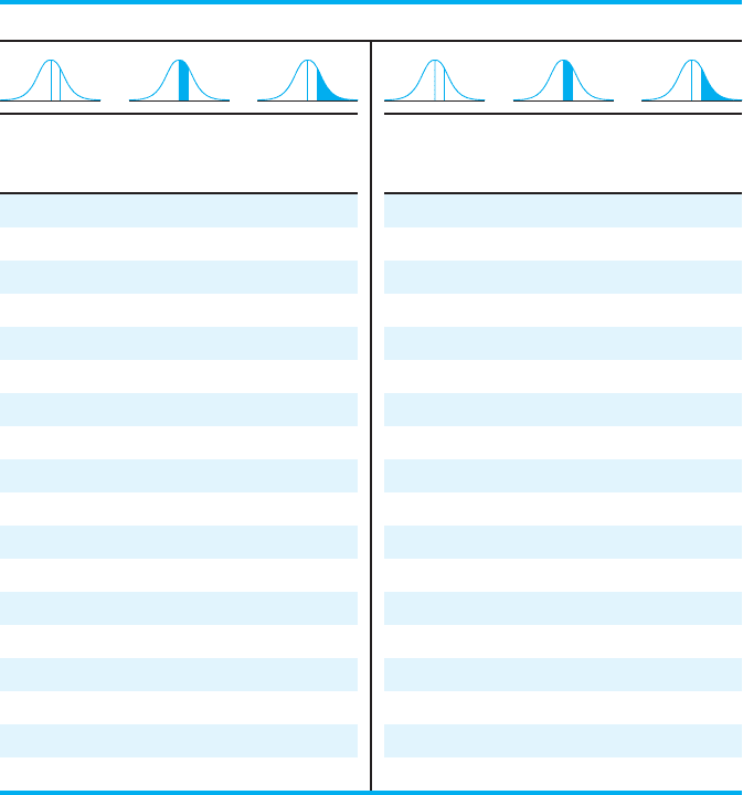
Take a look at Figure 5.7, which represents the area under the standard
normal curve in terms of standard deviations. Based on this figure, we see
that approximately 68% of the observations in the distribution fall between
1.0 and 1.0 standard deviations from the mean. This approximate per-
centage holds for all data that are normally distributed. Notice also that
approximately 13.5% of the observations fall between 1.0 and 2.0 and
another 13.5% between 1.0 and 2.0, and that approximately 2% of the
observations fall between 2.0 and 3.0 and another 2% between 2.0 and
3.0. Only 0.13% of the scores are beyond a z-score of 3.0. If we sum the
percentages in Figure 5.7, we have 100%—all of the area under the curve,
representing everybody in the distribution. If we sum half of the curve, we
have 50%—half of the distribution.
standard normal
distribution A normal
distribution with a mean of
0 and a standard deviation of 1.
standard normal
distribution A normal
distribution with a mean of
0 and a standard deviation of 1.
FIGURE 5.7
Area under the
standard normal
curve
34.13%
13.59%
2.15%
0.13%
2.15%
13.59%
34.13%
–3 –2 –1 0 1 32
Standard deviations
Frequency
0.13%
10017_05_ch5_p103-139.indd 126 2/1/08 1:19:07 PM
Data Organization and Descriptive Statistics
■ ■
127
With a curve that is normal or symmetrical, the mean, median, and mode
are all at the center point; thus, 50% of the scores are above this number, and
50% are below this number. This property helps us determine probabilities.
A probability is defined as the expected relative frequency of a particular
outcome. The outcome could be the result of an experiment or any situation
in which the result is not known in advance. For example, from the normal
curve, what is the probability of randomly choosing a score that falls above
the mean? The probability is equal to the proportion of scores in that area,
or .50. Figure 5.7 gives a rough estimate of the proportions under the normal
curve. Luckily for us, statisticians have determined the exact proportion of
scores that will fall between any two z-scores—for example, between z-scores
of 1.30 and 1.39. This information is provided in Table A.2 in Appendix A
at the back of the text. A small portion of this table is shown in Table 5.12.
probability The expected
relative frequency of a particular
outcome.
probability The expected
relative frequency of a particular
outcome.
0.00 .0000 .5000
0.01 .0040 .4960
0.02 .0080 .4920
0.03 .0120 .4880
0.04 .0160 .4840
0.05 .0199 .4801
0.06 .0239 .4761
0.07 .0279 .4721
0.08 .0319 .4681
0.09 .0359 .4641
0.10 .0398 .4602
0.11 .0438 .4562
0.12 .0478 .4522
0.13 .0517 .4483
0.14 .0557 .4443
0.15 .0596 .4404
0.16 .0636 .4364
0.17 .0675 .4325
0.18 .0714 .4286
0.19 .0753 .4247
0.20 .0793 .4207
0.21 .0832 .4268
0.22 .0871 .4129
0.23 .0910 .4090
0.24 .0948 .4052
0.25 .0987 .4013
0.26 .1026 .3974
0.27 .1064 .3936
0.28 .1103 .3897
0.29 .1141 .3859
0.30 .1179 .3821
0.31 .1217 .3783
0.32 .1255 .3745
0.33 .1293 .3707
0.34 .1331 .3669
0.35 .1368 .3632
TABLE 5.12 A Portion of the Standard Normal Curve Table
AREAS UNDER THE STANDARD NORMAL CURVE FOR VALUES OF z
AREA AREA
BETWEEN BEYOND
z MEAN AND z z
AREA AREA
BETWEEN BEYOND
z MEAN AND z z
(continued)
10017_05_ch5_p103-139.indd 127 2/1/08 1:19:07 PM
128
■ ■
CHAPTER 5
0.36 .1406 .3594
0.37 .1443 .3557
0.38 .1480 .3520
0.39 .1517 .3483
0.40 .1554 .3446
0.41 .1591 .3409
0.42 .1628 .3372
0.43 .1664 .3336
0.44 .1770 .3300
0.45 .1736 .3264
0.46 .1772 .3228
0.47 .1808 .3192
0.48 .1844 .3156
0.49 .1879 .3121
0.50 .1915 .3085
0.51 .1950 .3050
0.52 .1985 .3015
0.53 .2019 .2981
0.54 .2054 .2946
0.55 .2088 .2912
0.56 .2123 .2877
0.57 .2157 .2843
0.58 .2190 .2810
0.59 .2224 .2776
0.60 .2257 .2743
0.61 .2291 .2709
0.62 .2324 .2676
0.63 .2357 .2643
0.64 .2389 .2611
0.65 .2422 .2578
0.66 .2454 .2546
0.67 .2486 .2514
0.68 .2517 .2483
0.69 .2549 .2451
0.70 .2580 .2420
0.71 .2611 .2389
0.72 .2642 .2358
0.73 .2673 .2327
0.74 .2704 .2296
0.75 .2734 .2266
0.76 .2764 .2236
0.77 .2794 .2206
0.78 .2823 .2177
0.79 .2852 .2148
0.80 9.2881 .2119
0.81 .2910 .2090
0.82 .2939 .2061
0.83 .2967 .2033
TABLE 5.12 A Portion of the Standard Normal Curve Table (continued)
AREAS UNDER THE STANDARD NORMAL CURVE FOR VALUES OF z
AREA AREA
BETWEEN BEYOND
z MEAN AND z z
AREA AREA
BETWEEN BEYOND
z MEAN AND z z
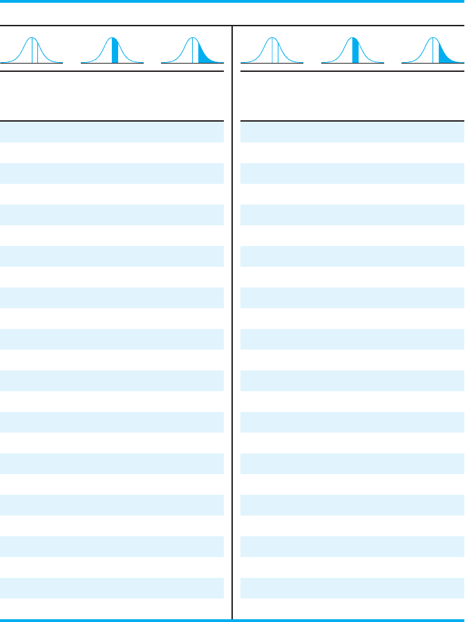
The columns across the top of the table are labeled z, Area Between Mean
and z, and Area Beyond z. There are also pictorial representations. The z
column refers to the z-score with which you are working. The Area Between
Mean and z is the area under the curve between the mean of the distribution
(where z 0) and the z-score with which you are working, that is, the pro-
portion of scores between the mean and the z-score in column 1. The Area
Beyond z is the area under the curve from the z-score out to the tail end of
the distribution. Notice that the entire table goes out to only a z-score of 4.00
10017_05_ch5_p103-139.indd 128 2/1/08 1:19:08 PM
Data Organization and Descriptive Statistics
■ ■
129
because it is very unusual for a normally distributed population of scores
to include scores larger than this. Notice also that the table provides infor-
mation about only positive z-scores, even though the distribution of scores
actually ranges from approximately 4.00 to 4.00. Because the distribution
is symmetrical, the areas between the mean and z and beyond the z-scores
are the same whether the z-score is positive or negative.
Let’s use some of the examples from earlier in the chapter to illustrate
how to use these proportions under the normal curve. Assume that the test
data described earlier (with
X 45 and S 4) are normally distributed, so
that the proportions under the normal curve apply. We calculated z-scores
for four individuals who took the test—Rich, Debbie, Pam, and Henry. Let’s
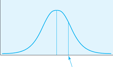
use Rich’s z-score to illustrate the use of the normal curve table. Rich had
a z-score equal to 1.00—1 standard deviation above the mean. Let’s begin
by drawing a picture representing the normal curve and then sketch in the
z-score. Thus, Figure 5.8 shows a representation of the normal curve, with a
line drawn at a z-score of 1.00.
Before we look at the proportions under the normal curve, we can begin
to gather information from this picture. We see that Rich’s score is above
the mean. Using the information from Figure 5.7, we see that roughly 34%
of the area under the curve falls between his z-score and the mean of the
distribution, whereas approximately 16% of the area falls beyond his z-score.
Using Table A.2 to get the exact proportions, we find (from the Area Beyond
z column) that the proportion of scores falling above the z-score of 1.0 is
.1587. This number can be interpreted to mean that 15.87% of the scores
were higher than Rich’s score, or that the probability of randomly choosing
a score with a z-score greater than 1.00 is .1587. To determine the propor-
tion of scores falling below Rich’s z-score, we need to use the Area Between
Mean and z column and add .50 to this proportion. According to the table,
the Area Between the Mean and the z-Score is .3413. Why must we add
.50 to this number? The table provides information about only one side of
the standard normal distribution. We must add in the proportion of scores
represented by the other half of the distribution, which is always .50. Look
back at Figure 5.8. Rich’s score is 1.00 above the mean, which means that
he did better than those between the mean and his z-score (.3413) and also
better than everybody below the mean (.50). Hence, 84.13% of the scores are
below Rich’s score.
+1.0
FIGURE 5.8
Standard normal
curve with z-score of
1.00 indicated
10017_05_ch5_p103-139.indd 129 2/1/08 1:19:08 PM
130
■ ■
CHAPTER 5
Let’s use Debbie’s z-score to further illustrate the use of the z table.
Debbie’s z-score was 0.00—right at the mean. We know that if she is at the
mean (z 0), then half of the distribution is below her score, and half is
above her score. Does this match what Table A.2 tells us? According to the
table, .5000 (50%) of scores are beyond this z-score, so the information in the
table does agree with our reasoning.
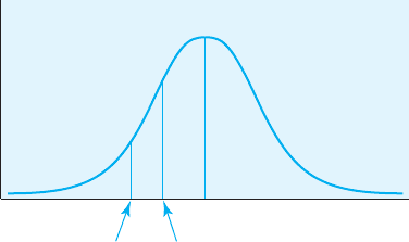
Using the z table with Pam and Henry’s z-scores is slightly more difficult
because both Pam and Henry had negative z-scores. Remember, Pam had a
z-score of 1.00, and Henry had a z-score of 1.50. Let’s begin by drawing
a normal distribution and then marking where both Pam and Henry fall on
that distribution. This information is represented in Figure 5.9.
Before even looking at the z table, let’s think about what we know from
Figure 5.9. We know that both Pam and Henry scored below the mean, that
they are in the lower 50% of the class, that the proportion of people scoring
higher than them is greater than .50, and that the proportion of people scor-
ing lower than them is less than .50. Keep this overview in mind as we use
Table A.2. Using Pam’s z-score of 1.0, see if you can determine the propor-
tion of scores lying above and below her score. If you determine that the pro-
portion of scores above hers is .8413 and that the proportion below is .1587,
then you are correct! Why is the proportion above her score .8413? We begin
by looking in the table at a z-score of 1.0 (remember, there are no negatives in
the table). The Area Between Mean and z is .3413, and then we need to add
the proportion of .50 in the top half of the curve. Adding these two propor-
tions, we get .8413. The proportion below her score is represented by the area
in the tail, the Area Beyond z of .1587. Note that the proportion above and
the proportion below should sum to 1.0 (.8413 .1587 1.0). Now see if you
can compute the proportions above and below Henry’s z-score of 1.5. Do
you get .9332 above his score and .0668 below his score? Good work!
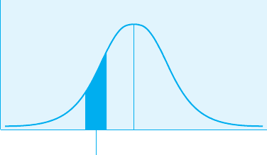
Now let’s try something slightly more difficult by determining the
proportion of scores that fall between Henry’s z-score of 1.5 and Pam’s
z-score of 1.0. Referring back to Figure 5.9, we see that we are targeting
the area between the two z-scores represented on the curve. Again, we
use Table A.2 to provide the proportions. The area between the mean and
Henry’s z-score of 1.5 is .4332, whereas the area between the mean and
Pam’s z-score of 1.0 is .3413. To determine the proportion of scores that
FIGURE 5.9
Standard normal
curve with z-scores
of 1.0 and 1.5
indicated
–1.0–1.5
10017_05_ch5_p103-139.indd 130 2/1/08 1:19:09 PM
Data Organization and Descriptive Statistics
■ ■
131
fall between the two, we subtract .3413 from .4332, obtaining a difference
of .0919. This result is illustrated in Figure 5.10.
The standard normal curve can also be used to determine an individual’s
percentile rank—the percentage of scores equal to or below the given raw
score, or the percentage of scores the individual’s score is higher than. To
determine a percentile rank, we must first know the individual’s z-score.
Let’s say we want to calculate an individual’s percentile rank based on
this person’s score on an intelligence test. The scores on the intelligence test
are normally distributed, with 100 and 15. Let’s suppose the indi-
vidual scored 119. Using the z-score formula, we have
z
X
______
119 100
_________
15
19
___
15
1.27
Looking at the Area Between Mean and z column for a score of 1.27,
we find the proportion .3980. To determine all of the area below the score, we
must add .50 to .3980; the entire area below a z-score of 1.27, then, is .8980.
If we multiply this proportion by 100, we can describe the intelligence test
score of 119 as being in the 89.80th percentile.
To practice calculating percentile ranks, see if you can calculate the per-
centile ranks for Rich, Debbie, Pam, and Henry from our previous examples.
You should arrive at the following percentile ranks.
Person Score (X) z-Score Percentile Rank
Rich 49 1.0 84.13th
Debbie 45 0.0 50.00th
Pam 41 1.0 15.87th
Henry 39 1.50 6.68th
Students most often have trouble determining percentile ranks from neg-
ative z-scores. Always draw a figure representing the normal curve with the
z-scores indicated; this will help you determine which column to use from
the z table. When the z-score is negative, the proportion of the curve repre-
senting those who scored lower than the individual (the percentile rank) is
found in the Area Beyond z column. When the z-score is positive, the propor-
tion of the curve representing those who scored lower than the individual
(the percentile rank) is found by using the Area Between Mean and z column
and adding .50 (the bottom half of the distribution) to this proportion.
percentile rank A score
that indicates the percentage of
people who scored at or below
a given raw score.
percentile rank A score
that indicates the percentage of
people who scored at or below
a given raw score.
FIGURE 5.10
Proportion of scores
between z-scores of
1.0 and 1.5
.0919
10017_05_ch5_p103-139.indd 131 2/1/08 1:19:09 PM