Hungerford T.W., Shaw D.J. Contemporary Precalculus: A Graphing Approach
Подождите немного. Документ загружается.

286 CHAPTER 4 Polynomial and Rational Functions
EXERCISES 4.4.A
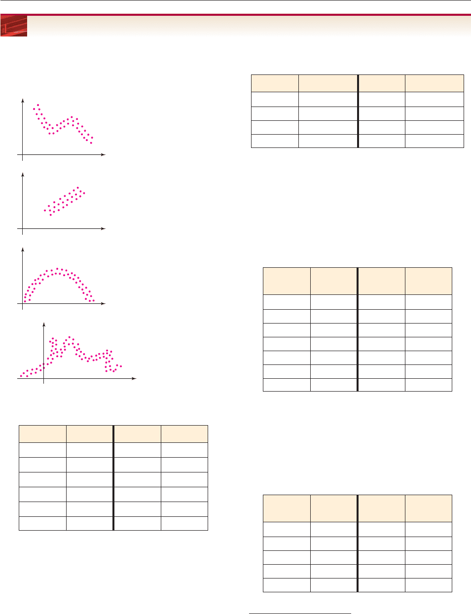
In Exercises 1–4, a scatter plot of data is shown. State the type
of polynomial model that seems most appropriate for the data
(linear, quadratic, cubic, or quartic). If none of them is likely to
provide a reasonable model, say so.
1.
2.
3.
4.
5. The table, which is based on the FBI Uniform Crime Reports,
shows the rate of property crime per 100,000 population.
(a) Use cubic regression to find a polynomial function that
models this data, with x 0 corresponding to 1990.
(b) According to this model, what was the property crime
rate in 1998 and 2001?
(c) The actual crime rates in 1998 and 2001 were 4052.5
and 3658.1 respectively. Was the model accurate?
(d) For how many years in the future is this model likely to
be a reasonable one?
x
y
x
y
x
y
x
y
6. The table shows actual and projected enrollment (in mil-
lions) in public high schools in selected years.*
(a) Use quartic regression to find a polynomial function
that models this data, with x 0 corresponding to 1975.
(b) According to the model, what was enrollment in 1998
and in 1999?
(c) Estimate the year between 1975 and 2000 in which
enrollment was the lowest. Does this estimate appear to
be accurate?
7. The table shows the air temperature at various times during
a spring day in Gainesville, Florida.
(a) Sketch a scatter plot of the data, with x 0 correspon-
ding to midnight.
(b) Find a quadratic polynomial model for the data.
(c) What is the predicted temperature for noon? For
9
A.M.? For 2 P.M.?
8. Right-fielder Bobby Abreu is an excellent batter. The fol-
lowing table shows his batting average for various years:
Year Crimes Year Crimes
1992 4903.7 1999 3743.6
1993 4740.0 2000 3618.3
1994 4660.2 2002 3630.6
1995 4590.5 2003 3591.2
1996 4451.0 2004 3514.2
1997 4316.3 2005 3429.8
Year Enrollment Year Enrollment
1975 14.3 1995 12.5
1980 13.2 2000 13.5
1985 12.4 2002 12.8
1990 11.3 2014 14.9
*U.S. National Center for Educational Statistics.
Temp Temp
Time (F°) Time (F°)
6 A.M.52 1 P.M.82
7 A.M.56 2 P.M.86
8 A.M.61 3 P.M.85
9 A.M.67 4 P.M.83
10 A.M.72 5 P.M.78
11 A.M.77 6 P.M.72
noon 80
Batting Batting
Year Average Year Average
1996 .227 2001 .289
1997 .250 2002 .308
1998 .312 2003
1999 .335 2004 .301
2000 .316 2005 .286
(a) Sketch a scatter plot of the data from 1996 to 2005, with
x 0 corresponding to 1996.
(b) Find a good polynomial model for this data.
(c) Use your model to estimate Bobby Abreu’s batting
average in 2003.
(d) Keeping in mind that baseball players’ batting averages
tend to decline as they get older, and that they tend to
stay above .100, how accurate do you think your model
would be if he were still playing baseball in 2016?
Why?
Use the following table in Exercises 9 and 10. It shows the
median income of U.S. households in constant 2004 dollars.*
9. (a) Sketch a scatter plot of the data from 1990 to 2004, with
x 0 corresponding to 1990 and y measured in thousands.
(b) Decide whether a quadratic or a cubic model seems
more appropriate and state its rule.
(c) Use the model to predict the median income in 2012.
(d) Does this model seem reasonable after 2012?
10. (a) Sketch a scatter plot of the data from 1994 to 2004, with
x 0 corresponding to 1994 and y measured in thou-
sands.
(b) Find both cubic and quartic models for this data.
(c) Is there any significant difference between the models
from 1994 to 2004? What about from 2004 to 2012?
(d) According to these models, when will the median in-
come reach $60,000?
11. The table shows the percentage of male high school stu-
dents who currently smoke cigarettes in various years.
†
(a) Sketch a scatter plot of the data, with x 0 correspon-
ding to 1990.
SPECIAL TOPICS 4.4.A Polynomial Models 287
(b) Find quadratic, cubic, and quartic polynomial models
for the data.
(c) Which model seems to fit this data best? Which one
seems most reasonable for future years.
12. The table shows the U.S. public debt per person (in dollars)
in selected years.*
(a) Sketch a scatter plot of the data.
(b) Find a quartic polynomial model for the data.
(c) Use the model to estimate the public debt per person in
1996. How does your estimate compare with the actual
figure of $19,805?
(d) Is this model likely to be accurate after 2003? Why?
13. (a) Find both a cubic and a quartic model for the data on the
number of unemployed people in the labor force in
Example 6 of Section 2.5.
(b) Does either model seem likely to be accurate in the
future?
14. The table shows the total advertising expenditures in the
United States (in billions of dollars) in selected years.
†
(a) Sketch a scatter plot of the data, with x 0 correspon-
ding to 1990.
(b) Find a quadratic model for the data.
(c) Use the model to estimate expenditures in 1995 and
2002.
(d) If this model remains accurate, when did expenditures
reach $350 billion?
Median Median
Year Income Year Income
1990 $42,086 1998 $43,659
1992 $41,043 2000 $45,730
1994 $40,439 2002 $45,222
1996 $41,722 2004 $44,473
Year Percent Year Percent
1991 27.6 1999 34.7
1993 29.8 2001 29.2
1995 35.4 2003 21.8
1997 37.7
Year Expenditures
1990 129.59
1992 132.65
1994 151.68
1996 175.23
1998 201.59
2000 236.33
*U.S. Census Bureau.
†
Youth at Risk Behavior Survey.
*U.S. Bureau of Public Debt.
†
Statistical Abstract of the United States: 2001.
Year Debit Year Debit
1981 $4,338 1993 $17,105
1983 $5,887 1995 $18,930
1985 $7,598 1997 $20,026
1987 $9,615 1999 $20,746
1989 $11,545 2001 $20.353
1991 $14,436 2003 $21,459

288 CHAPTER 4 Polynomial and Rational Functions
Domain
The domain of the rational function f (x)
g
h
(
(
x
x
)
)
is the set of all real numbers
that are not roots of the denominator h(x).
For instance, the domain of
f (x)
x
x
2
2
3
x
x
6
1
can be found by determining the roots of the denominator. It factors as
x
2
x 6 (x 2)(x 3),
so its roots are 2 and 3. Hence, the domain of f is the set of all real numbers
except 2 and 3.
The key to understanding the behavior of rational numbers is the following
fact from arithmetic.
The Big-Little
Principle
If c is a number far from 0, then 1/c is a number close to 0. Conversely, if
c is close to 0, then 1/c is far from 0. In less precise but more suggestive
terms:
b
1
ig
little and
lit
1
tle
big.
4.5 Rational Functions
■ Find the domain of a rational function.
■ Find the asymptotes of a linear rational function.
■ Analyze the graph of a rational function algebraically and
graphically.
■ Use rational functions to solve applied problems.
A rational function is a function whose rule is the quotient of two polynomials,
such as
f (x)
1
x
, t(x)
4
2
x
x
3
1
, k(x)
2
x
x
2
3
7
5
x
x
6
2
.
A polynomial function is defined for every real number, but the rational
function f (x) g(x)/h(x) is defined only when its denominator is nonzero.
Hence,
Section Objectives
For example, 5000 is big (far from 0), and 1/5000 is little (close to 0). Similarly,
1/1000 is very close to 0, but
1/
1
1000
1000
is far from 0. To see the role played by the Big-Little Principle, we examine two
rational functions that are part of the catalog of basic functions.
SECTION 4.5 Rational Functions 289
5
5
−5
−5
1
x
f(x) =
5
1
x
2
5
−5
−5
g(x) =
Figure 4–33
Figure 4–34
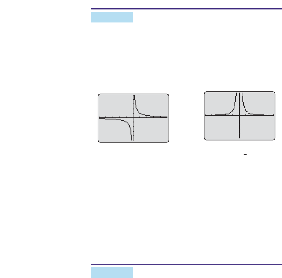
EXAMPLE 1
Reciprocal Functions Graph
f (x)
1
x
and g(x)
x
1
2
.
SOLUTION Note that f and g are not defined when x 0 (root of the denomi-
nator). The graphs are easily obtained, either by hand or by calculator (see Fig-
ures 4–33 and 4–34), and you should know their shapes by heart. ■
The Big-Little Principle explains why these graphs have the shapes they do.
When x is very close to 0, both 1/x and 1/x
2
are very far from 0. That’s why the
graphs “explode” near the undefined place at x 0, shooting sharply upward
or downward on either side of the y-axis. We say that the y-axis is the vertical
asymptote of the graph: The graph gets closer and closer to this line, but never
touches it. In a rational function, a vertical asymptote can occur only where the
function is not defined.
Similarly, when x is very far from 0, then 1/x and 1/x
2
are very small num-
bers. So the farther you go from the origin, the closer the graphs get to the line
y 0 (the x-axis), which is called the horizontal asymptote of the graph.
EXAMPLE 2
Without using technology, describe the graphs of
(a) h(x)
x
1
3
and (b) k(x)
x
2
4
1
x 4
.
SOLUTION
(a) Recall the graph of f (x)
1
x
in Figure 4–33, and note that
f (x 3)
x
1
3
h(x)
From Section 3.4, we know that the graph of h is the graph of f shifted horizon-
tally 3 units to the left, as shown in Figure 4–35(a) on the next page. The verti-
cal asymptote of this graph is at x 3 [the root of the denominator of h(x)].
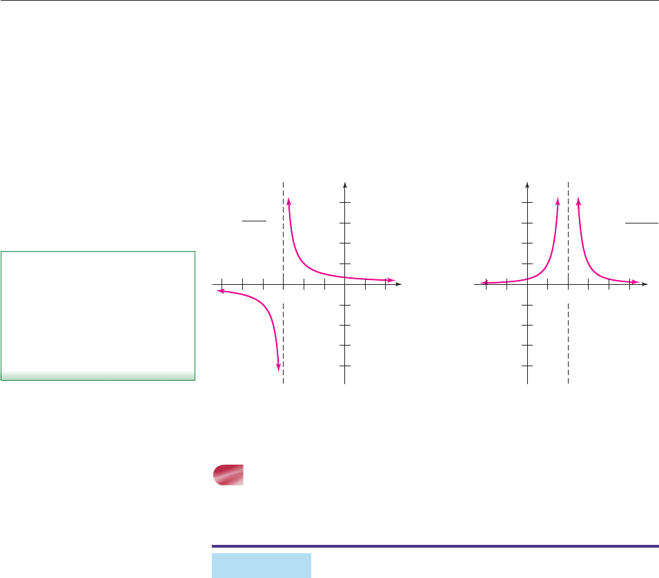
(b) To understand the graph of k, recall the graph of g(x)
x
1
2
in Figure 4–34
and factor the denominator of k(x):
k(x)
x
2
4
1
x 4
(x
1
2)
2
g(x 2).
Thus, the graph of k is the graph of g shifted horizontally 2 units to the right,
as shown in Figure 4–35(b). The vertical asymptote is at x 2 [the root of
the denominator of k(x)]. ■
290 CHAPTER 4 Polynomial and Rational Functions
x
y
2
3
4
1
−1
−2
−3
−4
−4 −3 −2−6 −5 −112
h(x) =
1
x + 3
(a)
x
y
2
3
4
1
−1
−2
−3
−4
12−2 −1354
k(x) =
1
(x − 2)
2
(b)
Figure 4–35
LINEAR RATIONAL FUNCTIONS
Next we consider the graphs of rational functions, where both the numerator and
denominator are either constants or first-degree polynomials.
EXAMPLE 3
Find the asymptotes of the graph of
f (x)
2
x
x
1
4
and graph the function.
SOLUTION The function is not defined when x 2 because the denominator
is 0 there. When x is a number very close to 2, then
the numerator x 1 is very close to 3;
the denominator 2x 4 is very close to 0.
Therefore,
f (x)
2
x
x
1
4
lit
3
tle
BIG (far from 0).
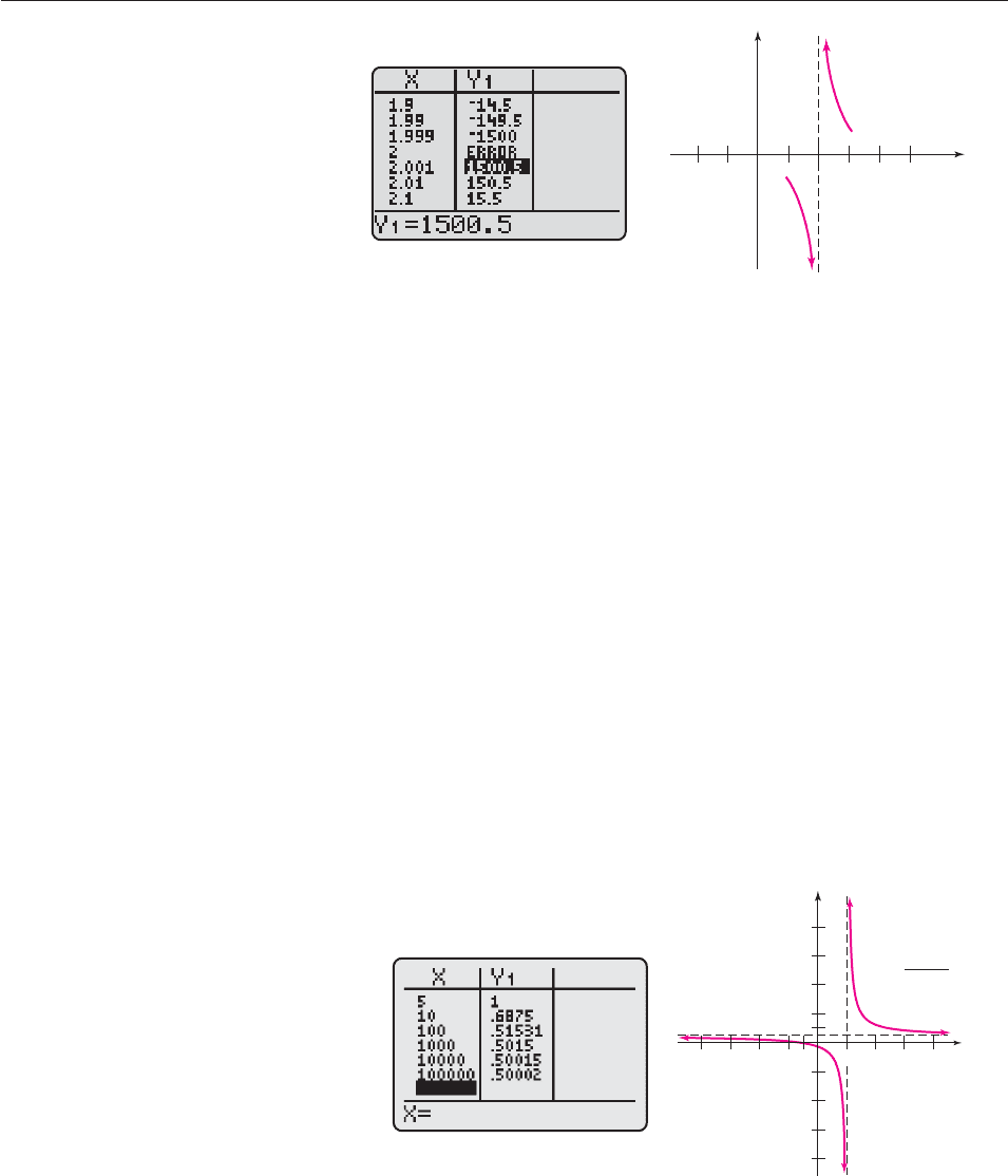
Consequently, the graph explodes near x 2, as shown in the table and partial
graph in Figure 4–36. The vertical line x 2 is the vertical asymptote of the graph.
NOTE
The asymptotes are shown as dashed
lines in Figure 4–35 and in the figures
below. The asymptotes are included for
easier visualization, but they are not
part of the graph.
To determine the horizontal asymptote of the graph, we rewrite the rule of f
like this:
f (x)
2
x
x
1
4
.
As x gets larger in absolute value (far from 0), both 1/x and 4/x get very close to
0 by the Big-Little Principle. Consequently,
f (x)
1
2
(
(
1
4
/
/
x
x
)
)
gets very close to
1
2
0
0
1
2
.
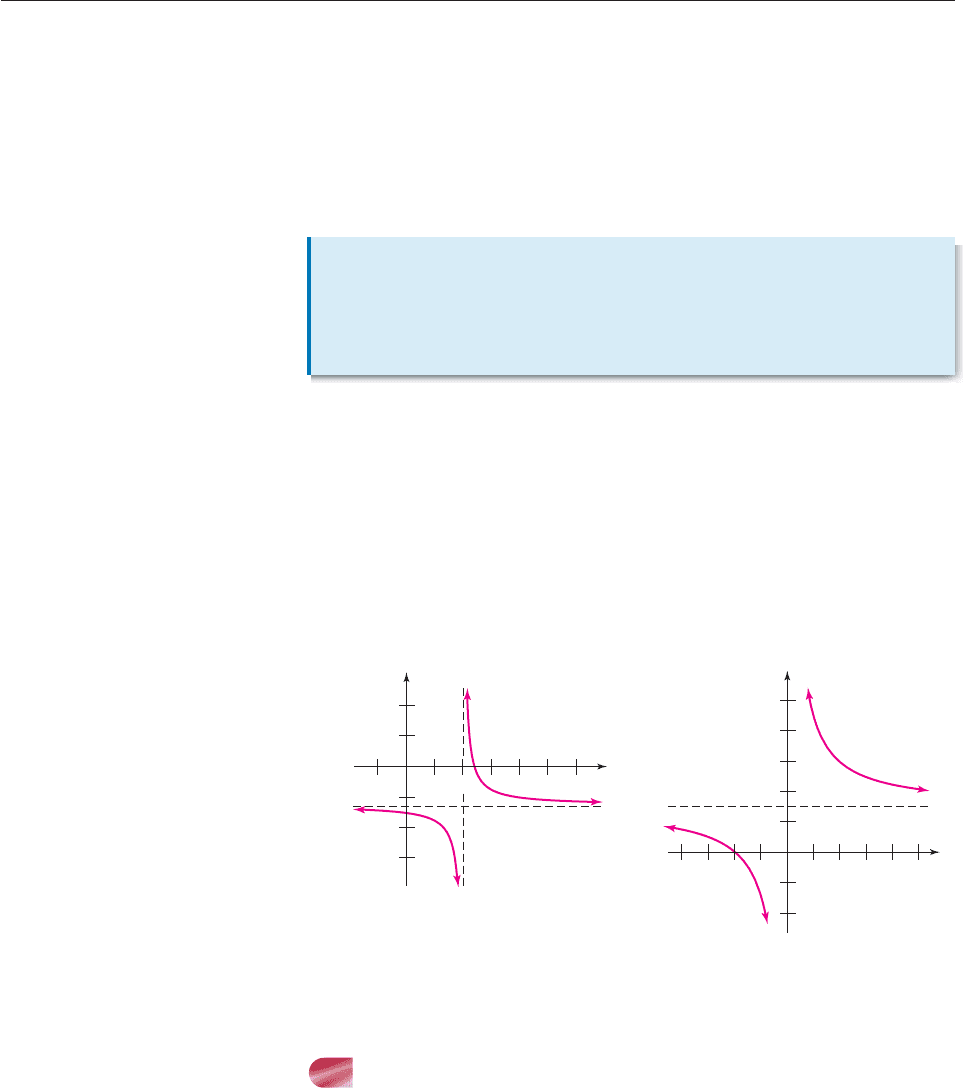
So when x is large, the graph gets closer and closer to the horizontal line
y 1/2, but never touches it, as shown in Figure 4 –37. Thus, the line y 1/2 is
the horizontal asymptote of the graph.
The preceding information, together with a few hand-plotted points, pro-
duces the graph in Figure 4–37.
1
1
x
2
4
x
x
x
1
2x
x
4
SECTION 4.5 Rational Functions 291
x
y
Figure 4–36
x
y
4
6
8
2
−2
−4
−6
−8
1
−8 −6 −4 −224
f(x) =
x + 1
2x − 4
6−1
Figure 4–37
We can see this result in a different way. When x is very large, we can make the
approximations x 1 x and 2x 4 2x. Therefore, we have, for large x,
f (x)
2
x
x
1
4
2
x
x
1
2
. ■
We can generalize the process used at the end of Example 3. If f(x)
a
cx
x
d
b
,
with a and c non-zero, then for large x:
a
cx
x
d
b
a
cx
x
a
c
.
We summarize below:
292 CHAPTER 4 Polynomial and Rational Functions
Linear Rational
Functions
The graph of f (x)
a
cx
x
d
b
(with c 0 and ad bc) has two asymptotes:
The vertical asymptote occurs at the root of the denominator.
The horizontal asymptote is the line y a/c.
x
y
4
2
8
6
−2
−3 −2 −11234
(b)
x
y
4
2
−2
−4
−6
−1123456
(a)
Figure 4–38
RATIONAL FUNCTIONS AND TECHNOLOGY
Getting an accurate graph of a rational function on a calculator often depends on
choosing an appropriate viewing window. For example, a TI-83+ produced the
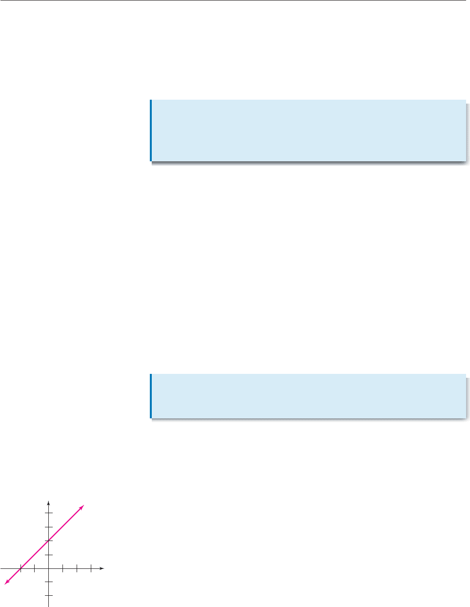
following graphs of
f(x)
2
x
x
1
4
in Figure 4–39, two of which do not look like Figure 4–37 as they should.
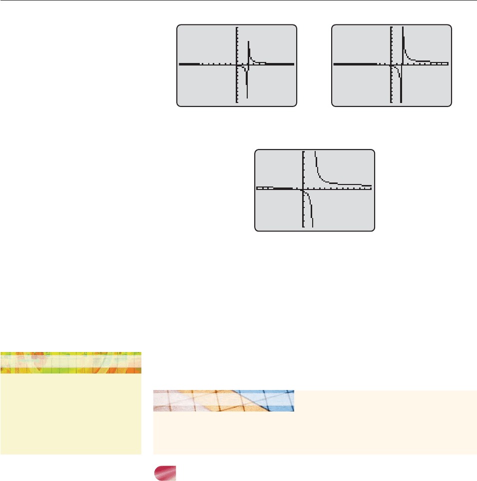
Figure 4–38 shows some additional examples.
f (x)
2
5
x
x
4
12
k(x)
3x
x
6
3
1
x
x
6
0
Vertical asymptote x 2 Vertical asymptote x 0
Horizontal asymptote y
5
2
Horizontal asymptote y
3
1
3
SECTION 4.5 Rational Functions 293
20
10
−10
−20
10
10
−10
−10
(
a
)(
b
)
6
12
−8
−6
(
c
)
Figure 4–39
The vertical segments in graphs (a) and (b) are not representations of the vertical
asymptote. They are a result of the calculator evaluating f (x) just to the left of
x 2 and just to the right of x 2 but not at x 2 and then erroneously con-
necting these points with a near vertical segment that looks like an asymptote.
In the accurate graph (c), the calculator attempted to plot a point with x 2
and, when it found that f (2) was not defined, skipped a pixel and did not join the
points on either side of the skipped one.
TECHNOLOGY TIP
To avoid erroneous vertical lines, use a
window with the vertical asymptote in
the center, as in Figure 4–39(c) (where
the asymptote at x 2 is half-way
between 8 and 12). Also see the
Technology Tip on page 298.
Find a viewing window that displays the graph of f (x) in Figure 4–38(a), without
any erroneous vertical line segments being shown. The Technology Tip in the
margin may be helpful.
GRAPHING EXPLORATION
PROPERTIES OF RATIONAL GRAPHS
Here is a summary of the important characteristics of graphs of more complicated
rational functions.
CONTINUITY AND SMOOTHNESS
There will be breaks in the graph of a rational function wherever the function is
not defined. Between those breaks, the graph is a continuous unbroken curve. In
addition, the graph has no sharp corners.
LOCAL MAXIMA AND MINIMA
The graph may have some local extrema (peaks and valleys), and calculus is
needed to determine their exact location. There are no simple rules for the possi-
ble number of peaks and valleys as there were with polynomial functions.
INTERCEPTS
As with any function, the y-intercept of the graph of a rational function f occurs
at f (0), provided that f is defined at x 0. The x-intercepts of the graph of any
function f occur at each number c for which f (c) 0. Now a fraction is 0 only
when its numerator is 0 and its denominator is nonzero (since division by 0 is not
defined). Thus,
294 CHAPTER 4 Polynomial and Rational Functions
Intercepts
The x-intercepts of the graph of the rational function f (x)
g
h
(
(
x
x
)
)
occur at the
numbers that are roots of the numerator g(x) but not of the denominator h(x).
If f has a y-intercept, it occurs at f (0).
For example, the graph of
f (x)
x
2
x
x
5
2
has x-intercepts at x 1 and x 2 [which are the roots of x
2
x 2
(x 1)(x 2), but not of x 5] and y-intercept at y 2/5 (the value of f at
x 0).
VERTICAL ASYMPTOTES
In Example 3, we saw that the graph of
f (x)
2
x
x
1
4
had a vertical asymptote at x 2. Note that x 2 is a root of the denominator
2x 4, but not of the numerator x 1. The same thing occurs in the general case.
Vertical
Asymptotes
The function f (x)
g
h
(
(
x
x
)
)
has a vertical asymptote at every number that is a
root of the denominator h(x), but not of the numerator g(x).
HOLES
When simplifying rational expressions, we often cancel factors, like so:
x
x
2
2
4
(x
x
2
)(x
2
2)
x 2.
But the functions given by
p(x)
x
x
2
2
4
and q(x) x 2
are not the same, because when x 2,
q(2) 2 2 4, but p(2)
2
2
2
2
2
0
0
,
which is not defined. For any number other than 2, the two functions do have
the same value, and hence, the same graph. The graph of q(x) x 2 is a straight
line that includes the point (2, 4), as shown in Figure 4–40. The graph of p(x) is
x
y
−2 −1 123
−2
4
2
Figure 4–40
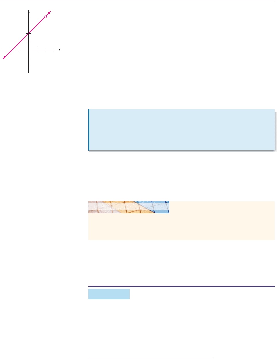
the same straight line, but with the point (2, 4) omitted, so that the graph of p has
a hole at x 2 (indicated by an open circle in Figure 4–41). Note that the hole
occurs at x 2, which is a root of multiplicity 1 in both the numerator and the
denominator of
p(x)
x
x
2
2
4
(x
x
2
)(x
2
2)
.*
Similarly, the graph of g(x)
x
x
2
3
is the same as the graph of f (x)
1
x
, except
at x 0, where neither function is defined. In this case, however, there is a verti-
cal asymptote rather than a hole at x 0 (see Figure 4 –33 on page 289). Note
that the vertical asymptote occurs at x 0, which is a root of multiplicity 2 in the
numerator, but of larger multiplicity 3 in the denominator. In general,
SECTION 4.5 Rational Functions 295
x
y
−2 123
−2
4
2
Figure 4–41
Holes
Let f (x)
g
h
(
(
x
x
)
)
be a rational function and d a root of both g(x) and h(x). If
the multiplicity of d as a root of g(x) is greater than or equal to its multi-
plicity as a root of h(x), then the graph of f has a hole at x d. Otherwise,
the graph has a vertical asymptote at x d.
A calculator-drawn graph may not show holes where it should. If the cal-
culator actually attempts to compute an undefined quantity, it indicates a hole
by skipping a pixel; otherwise, it may erroneously show a continuous graph
with no hole.
Graph p(x)
x
x
2
2
4
with various viewing windows. Does your calculator display
the hole at x 2?
GRAPHING EXPLORATION
BEHAVIOR WHEN x IS LARGE
The shape of a rational graph at the far left and far right (that is, when x is large)
can usually be found by algebraic analysis, as in the next example.
EXAMPLE 4
Determine the shape of the graph when x is large for the following functions.
(a) f (x)
7x
4
2x
4
6
x
3
x
2
4
(b) g(x)
x
3
3
x
x
2
2
2
x 3
(c) h(x)
2
x
x
3
3
5
*Multiplicity of roots was discussed on page 273.
