Hjorth-Jensen M. Computational Physics

Подождите немного. Документ загружается.

9.6. MONTE CARLO INTEGRATION OF MULTIDIMENSIONAL INTEGRALS 159

9.6.1 Brute force integration

#include < iostream >

#include < fstream >

#include < iomanip >

#include

using namespace std ;

double brute_force_MC ( double ) ;

/ / Main fun ctio n begins here

int main ()

{

int n ;

double x [6 ] , y , fx ;

double int_mc = 0 . ; double variance = 0 . ;

double sum_sigma = 0 . ; long idum = 1 ;

double length = 5 . ; / / we f i x the max si z e of the box to L=5

double volume=pow((2 length ) ,6) ;

cout < < < < endl ;

cin > > n ;

/ / evaluate the i n t egr a l with importance sampling

for ( int i = 1 ; i <= n ; i ++){

/ / x [ ] contains the random numbers for a l l dimensions

for ( int j = 0 ; j < 6 ; j ++) {

x[ j ]= length +2 length ran0 (&idum ) ;

}

fx=brute_force_MC (x ) ;

int_mc += fx ;

sum_sigma += fx fx ;

}

int_mc = int_mc / ( ( double ) n ) ;

sum_sigma = sum_sigma / ( ( double ) n ) ;

variance =sum_sigma int_mc int_mc ;

/ / f i n a l output

cout < < s e t i o s f l a g s ( ios : : showpoint | ios : : uppercase ) ;

cout < < < < setw (10) < < s e t p re cisi on (8)

< < volume int_mc ;

cout < < < < setw (10) < < se t p r e c i s i o n (8) < < volume s q r t

( variance / ( ( double ) n ) ) < < endl ;

return 0 ;

} / / end of main program

/ / t hi s fun ctio n d efin es the integrand to i n teg r ate

double brute_force_MC ( double x )

160 CHAPTER 9. OUTLINE OF THE MONTE-CARLO STRATEGY

{

double a = 1 . ; double b = 0 . 5 ;

/ / evaluate the d i f f e r e n t terms of the exponential

double xx=x [0] x [0]+ x [1] x [1]+ x [2] x [2] ;

double yy=x [3] x [3]+ x [4] x [4]+ x [5] x [5] ;

double xy=pow ( ( x[0] x [3 ] ) ,2) +pow ( ( x[1] x [4 ]) ,2)+pow ( ( x[2] x [5 ]) ,2) ;

return exp( a xx a yy b xy ) ;

} / / end f un ct ion for the integrand

9.6.2 Importance sampling

This code includes a call to the function

_ , which produces random numbers

from a gaussian distribution. .

/ / importance sampling with gaussian deviates

#include < iostream >

#include < fstream >

#include < iomanip >

#include

using namespace std ;

double gaussian_MC ( double ) ;

double g aussian_deviate ( long ) ;

/ / Main fun ctio n begins here

int main ()

{

int n ;

double x [6 ] , y , fx ;

cout < < < < endl ;

cin > > n ;

double int_mc = 0 . ; double variance = 0 . ;

double sum_sigma = 0 . ; long idum = 1 ;

double length = 5 . ; / / we f i x the max si z e of the box to L=5

double volume=pow( acos ( 1.) , 3. ) ;

double s qrt2 = 1 . / s qr t ( 2 . ) ;

/ / evaluate the i n t egr a l with importance sampling

for ( int i = 1 ; i <= n ; i ++){

/ / x [ ] contains the random numbers for a l l dimensions

for ( int j = 0 ; j < 6; j ++) {

x [ j ] = g aussian_deviate (&idum ) s qrt2 ;

}

fx=gaussian_MC ( x ) ;

int_mc += fx ;

sum_sigma += fx fx ;

}

9.6. MONTE CARLO INTEGRATION OF MULTIDIMENSIONAL INTEGRALS 161

int_mc = int_mc / ( ( double ) n ) ;

sum_sigma = sum_sigma / ( ( double ) n ) ;

variance =sum_sigma int_mc int_mc ;

/ / f i n a l output

cout < < s e t i o s f l a g s ( ios : : showpoint | ios : : uppercase ) ;

cout < < < < setw (10) < < s e t p re cisi on (8)

< < volume int_mc ;

cout < < < < setw (10) < < se t p r e c i s i o n (8) < < volume s q r t

( variance / ( ( double ) n ) ) < < endl ;

return 0 ;

} / / end of main program

/ / t hi s fun ctio n d efin es the integrand to i n teg r ate

double gaussian_MC ( double x )

{

double a = 0 . 5 ;

/ / evaluate the d i f f e r e n t terms of the exponential

double xy=pow ( ( x[0] x [3 ] ) ,2) +pow ( ( x[1] x [4 ]) ,2)+pow ( ( x[2] x [5 ]) ,2) ;

return exp( a xy ) ;

} / / end f un ct ion for the integrand

/ / random numbers with gaussian d i s t r i b u t i o n

double g aussian_deviate ( long idum )

{

s ta ti c int i s e t = 0;

s ta ti c double gset ;

double fac , rsq , v1 , v2 ;

i f ( idum < 0) i s e t =0;

i f ( i s e t == 0) {

do {

v1 = 2 . ran0 ( idum ) 1.0;

v2 = 2 . ran0 ( idum ) 1.0;

rsq = v1 v1+v2 v2 ;

} while ( rsq > = 1 . 0 | | rsq = = 0 . ) ;

fac = s qr t ( 2. log ( rsq ) / rsq ) ;

gset = v1 fac ;

i s e t = 1 ;

return v2 fac ;

} else {

i s e t =0;

return gset ;

}

} / / end f un ct ion for gaussian de viat es

Chapter 10

Random walks and the Metropolis

algorithm

10.1 Motivation

In the previous chapter we discussed technical aspects of Monte Carlo integration such as algo-

rithms for generating random numbers and integration of multidimensional integrals. The latter

topic served to illustrate two key topics in Monte Carlo simulations, namely a proper selection

of variables and importance sampling. An intelligent selection of variables, good sampling tech-

niques and guiding functions can be crucial for the outcome of our Monte Carlo simulations.

Examples of this will be demonstrated in the chapters on statistical and quantum physics appli-

cations. Here we make a detour however from this main area of applications. The focus is on

diffusion and random walks. The rationale for this is that the tricky part of an actual Monte Carlo

simulation resides in the appropriate selection of random states, and thereby numbers, according

to the probability distribution (PDF) at hand. With appropriate there is however much more to

the picture than meets the eye.

Suppose our PDF is given by the well-known normal distribution. Think of for example the

velocity distribution of an ideal gas in a container. In our simulations we could then accept or

reject new moves with a probability proportional to the normal distribution. This would parallel

our example on the sixth dimensional integral in the previous chapter. However, in this case

we would end up rejecting basically all moves since the probabilities are exponentially small in

most cases. The result would be that we barely moved from the initial position. Our statistical

averages would then be signiﬁcantly biased and most likely not very reliable.

Instead, all Monte Carlo schemes used are based on Markov processes in order to generate

new random states. A Markov process is a random walk with a selected probability for making a

move. The new move is independent of the previous history of the system. The Markov process

is used repeatedly in Monte Carlo simulations in order to generate new random states. The

reason for choosing a Markov process is that when it is run for a long enough time starting with

a random state, we will eventually reach the most likely state of the system. In thermodynamics,

this means that after a certain number of Markov processes we reach an equilibrium distribution.

163

164 CHAPTER 10. RANDOM WALKS AND THE METROPOLIS ALGORITHM

This mimicks the way a real system reaches its most likely state at a given temperature of the

surroundings.

To reach this distribution, the Markov process needs to obey two important conditions, that

of ergodicity and detailed balance. These conditions impose then constraints on our algorithms

for accepting or rejecting new random states. The Metropolis algorithm discussed here abides to

both these constraints and is discussed in more detail in Section 10.4. The Metropolis algorithm

is widely used in Monte Carlo simulations of physical systems and the understanding of it rests

within the interpretation of random walks and Markov processes. However, before we do that we

discuss the intimate link between random walks, Markov processes and the diffusion equation. In

section 10.3 we showthat a Markov process is nothing but the discretized version of the diffusion

equation. Diffusion and random walks are discussed from a more experimental point of view in

the next section. There we show also a simple algorithm for random walks and discuss eventual

physical implications.

10.2 Diffusion equation and random walks

Physical systems subject to random inﬂuences from the ambient have a long history, dating

back to the famous experiments by the British Botanist R. Brown on pollen of different plants

dispersed in water. This lead to the famous concept of Brownian motion. In general, small

fractions of any system exhibit the same behavior when exposed to random ﬂuctuations of the

medium. Although apparently non-deterministic, the rules obeyed by such Brownian systems

are laid out within the framework of diffusion and Markov chains. The fundamental works on

Brownian motion were developed by A. Einstein at the turn of the last century.

Diffusion and the diffusion equation are central topics in both Physics and Mathematics, and

their ranges of applicability span from stellar dynamics to the diffusion of particles governed by

Schrödinger’s equation. The latter is, for a free particle, nothing but the diffusion equation in

complex time!

Let us consider the one-dimensional diffusion equation. We study a large ensemble of parti-

cles performing Brownian motion along the

-axis. There is no interaction between the particles.

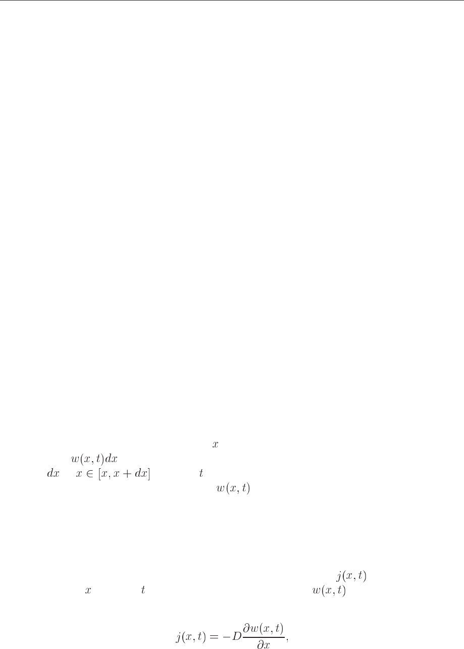
We deﬁne as the probability of ﬁnding a given number of particles in an interval

of length

in at a time . This quantity is our probability distribution function

(PDF). The quantum physics equivalent of is the wave function itself. This diffusion

interpretation of Schrödinger’s equation forms the starting point for diffusion Monte Carlo tech-

niques in quantum physics.

10.2.1 Diffusion equation

From experiment there are strong indications that the ﬂux of particles

, viz., the number of

particles passing

at a time is proportional to the gradient of . This proportionality is

expressed mathematically through

(10.1)

10.2. DIFFUSION EQUATION AND RANDOM WALKS 165

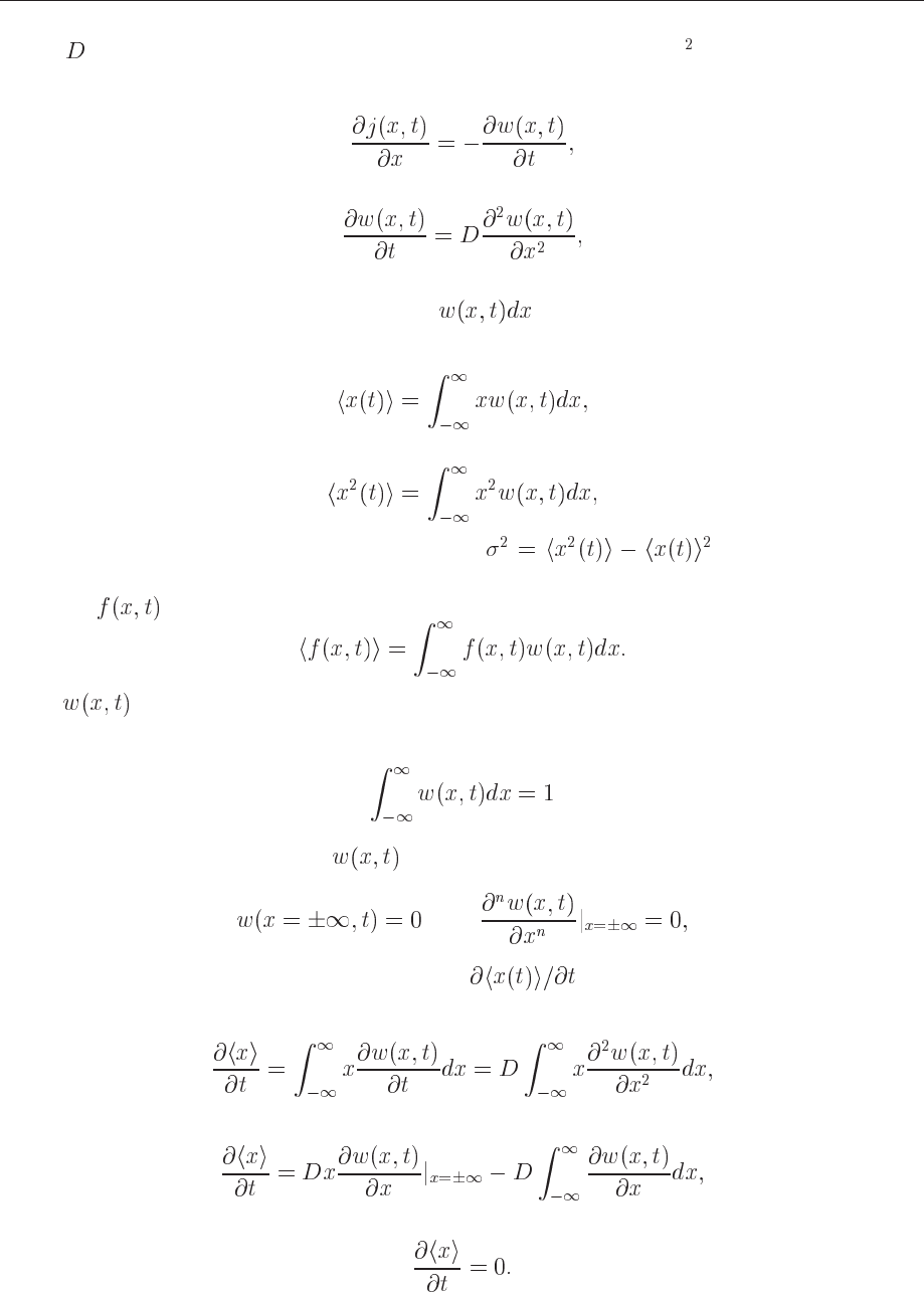
where is the so-called diffusion constant, with dimensionality length per time. If the number

of particles is conserved, we have the continuity equation

(10.2)

which leads to

(10.3)

which is the diffusion equation in one dimension.

With the probability distribution function

we can use the results from the previous

chapter to compute expectation values such as the mean distance

(10.4)

(10.5)

which allows for the computation of the variance

. Note well that these

expectation values are time-dependent. In a similar way we can also deﬁne expectation values of

functions as

(10.6)

Since

is now treated as a PDF, it needs to obey the same criteria as discussed in the

previous chapter. However, the normalization condition

(10.7)

imposes signiﬁcant constraints on

. These are

(10.8)

implying that when we study the time-derivative

, we obtain after integration by parts

and using Eq. (10.3)

(10.9)

leading to

(10.10)

implying that

(10.11)

166 CHAPTER 10. RANDOM WALKS AND THE METROPOLIS ALGORITHM

This means in turn that is independent of time. If we choose the initial position ,

the average displacement

. If we link this discussion to a random walk in one dimension

with equal probability of jumping to the left or right and with an initial position , then

our probability distribution remains centered around as function of time. However, the

variance is not necessarily 0. Consider ﬁrst

(10.12)

where we have performed an integration by parts as we did for

. A further integration by

parts results in

(10.13)

leading to

(10.14)

and the variance as

(10.15)

The root mean square displacement after a time is then

(10.16)

This should be contrasted to the displacement of a free particle with initial velocity

. In that

case the distance from the initial position after a time is whereas for a diffusion

process the root mean square value is

. Since diffusion is strongly linked

with random walks, we could say that a random walker escapes much more slowly from the

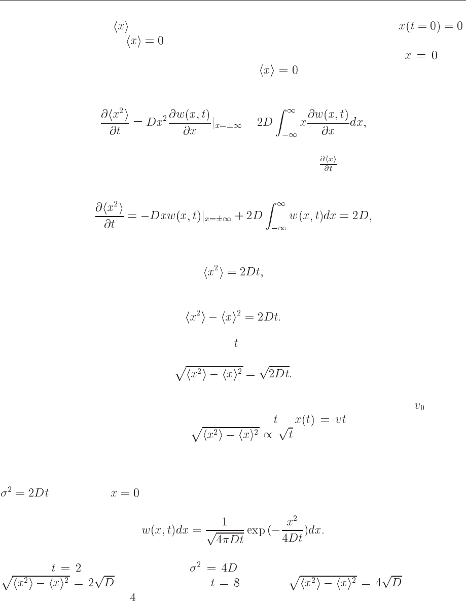
starting point than would a free particle. We can vizualize the above in the following ﬁgure. In

Fig. 10.1 we have assumed that our distribution is given by a normal distribution with variance

, centered at . The distribution reads

(10.17)

At a time

s the new variance is s, implying that the root mean square value is

. At a further time we have . While time

has elapsed by a factor of

, the root mean square has only changed by a factor of 2. Fig. 10.1

demonstrates the spreadout of the distribution as time elapses. A typical example can be the

diffusion of gas molecules in a container or the distribution of cream in a cup of coffee. In both

cases we can assume that the the initial distribution is represented by a normal distribution.

10.2. DIFFUSION EQUATION AND RANDOM WALKS 167

Figure 10.1: Time development of a normal distribution with variance and with

m /s. The solid line represents the distribution at s while the dotted line stands for

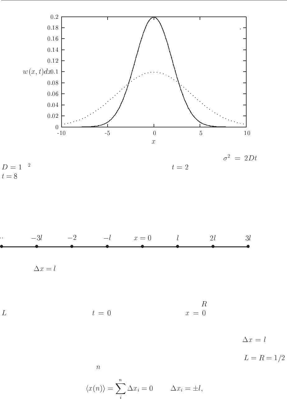
Figure 10.2: One-dimensional walker which can jump either to the left or to the right. Every step

has length

10.2.2 Random walks

Consider now a random walker in one dimension, with probability of moving to the right and

for moving to the left. At we place the walker at , as indicated in Fig. 10.2.

The walker can then jump, with the above probabilities, either to the left or to the right for each

time step. Note that in principle we could also have the possibility that the walker remains in the

same position. This is not implemented in this example. Every step has length

. Time

is discretized and we have a jump either to the left or to the right at every time step. Let us now

assume that we have equal probabilities for jumping to the left or to the right, i.e.,

The average displacement after time steps is

(10.18)

168 CHAPTER 10. RANDOM WALKS AND THE METROPOLIS ALGORITHM

since we have an equal probability of jumping either to the left or to right. The value of

(10.19)

For many enough steps the non-diagonal contribution is

(10.20)

since

. The variance is then

(10.21)

It is also rather straightforward to compute the variance for

. The result is

(10.22)

In Eq. (10.21) the variable

represents the number of time steps. If we deﬁne , we can

then couple the variance result from a random walk in one dimension with the variance from the

diffusion equation of Eq. (10.15) by deﬁning the diffusion constant as

(10.23)

In the next section we show in detail that this is the case.

The program below demonstrates the simplicity of the one-dimensional random walk algo-

rithm. It is straightforward to extend this program to two or three dimensions as well. The input

is the number of time steps, the probability for a move to the left or to the right and the total

number of Monte Carlo samples. It computes the average displacement and the variance for one

random walker for a given number of Monte Carlo samples. Each sample is thus to be consid-

ered as one experiment with a given number of walks. The interesting part of the algorithm is

described in the function mc_sampling. The other functions read or write the results from screen

or ﬁle and are similar in structure to programs discussed previously. The main program reads the

name of the output ﬁle from screen and sets up the arrays containing the walker’s position after

a given number of steps.

programs/chap10/program1.cpp

1 dim random walk program .

A walker makes several t r i a l s step s with

a given number of walks per t r i a l

#include < iostream >

#include < fstream >