Hjorth-Jensen M. Computational Physics

Подождите немного. Документ загружается.

9.5. IMPROVED MONTE CARLO INTEGRATION 149

The second term on the rhs disappears since this is just the mean and employing the deﬁnition of

we have

(9.59)

resulting in

(9.60)

and in the limit we obtain

(9.61)

which is the normal distribution with variance

, where is the variance of the PDF

and is also the mean of the PDF .

Thus, the central limit theorem states that the PDF

of the average of random values

corresponding to a PDF is a normal distribution whose mean is the mean value of the PDF

and whose variance is the variance of the PDF divided by , the number of values

used to compute

The theorem is satisﬁed by a large class of PDFs. Note however that for a ﬁnite

, it is not

always possible to ﬁnd a closed expression for .

9.5 Improved Monte Carlo integration

In section 5.1 we presented a simple brute force approach to integration with the Monte Carlo

method. There we sampled over a given number of points distributed uniformly in the interval

with the weights .

Here we introduce two important topics which in most cases improve upon the above simple

brute force approach with the uniform distribution

for . With improvements

we think of a smaller variance and the need for fewer Monte Carlo samples, although each new

Monte Carlo sample will most likely be more times consuming than corresponding ones of the

brute force method.

The ﬁrst topic deals with change of variables, and is linked to the cumulativefunction

of a PDF . Obviously, not all integration limits go from to , rather, in

physics we are often confronted with integration domains like

etc. Since all random number generators give numbers in the interval , we need a

mapping from this integration interval to the explicit one under consideration.

150 CHAPTER 9. OUTLINE OF THE MONTE-CARLO STRATEGY

The next topic deals with the shape of the integrand itself. Let us for the sake of simplicity

just assume that the integration domain is again from

to . If the function to

be integrated has sharp peaks and is zero or small for many values of , most

samples of givecontributionsto the integral which are negligible. As a consequence

we need many

samples to have a sufﬁcient accuracy in the region where is peaked.

What do we do then? We try to ﬁnd a new PDF chosen so as to match in order

to render the integrand smooth. The new PDF

has in turn an domain which most

likely has to be mapped from the domain of the uniform distribution.

Why care at all and not be content with just a change of variables in cases where that is

needed? Below we show several examples of how to improve a Monte Carlo integration through

smarter choices of PDFs which render the integrand smoother. However one classic example

from quantum mechanics illustrates the need for a good sampling function.

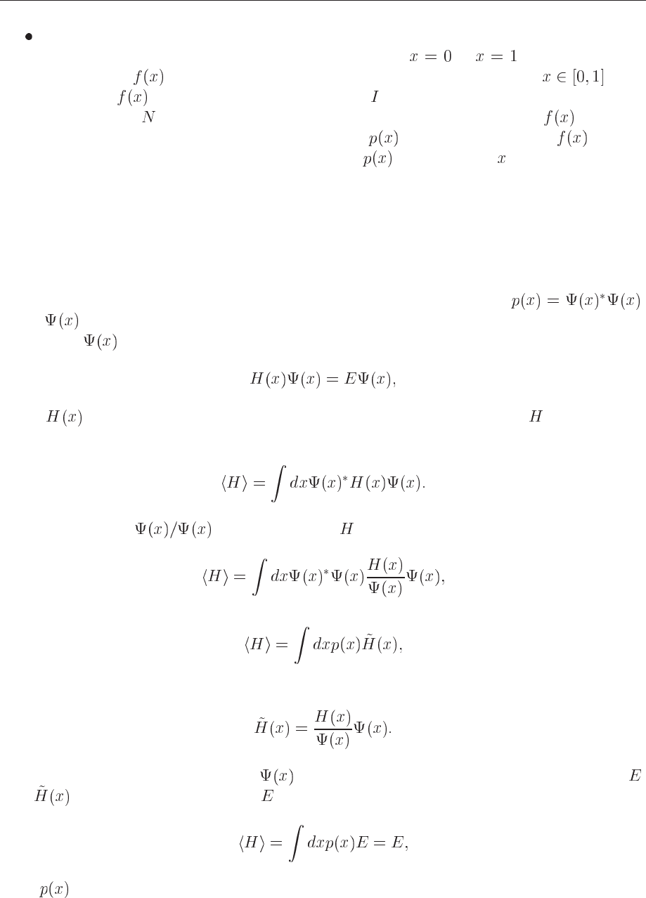
In quantum mechanics, the probability distribution function is given by ,

where is theeigenfunction arising from the solutionof e.g., the time-independentSchrödinger

equation. If

is an eigenfunction, the corresponding energy eigenvalue is given by

(9.62)

where is the hamiltonian under consideration. The expectation value of , assuming that

the quantum mechanical PDF is normalized, is given by

(9.63)

We could insert right to the left of and rewrite the last equation as

(9.64)

(9.65)

which is on the form of an expectation value with

(9.66)

The crucial point to note is that if

is the exact eigenfunction itself with eigenvalue ,

then

reduces just to the constant and we have

(9.67)

since

is normalized.

9.5. IMPROVED MONTE CARLO INTEGRATION 151

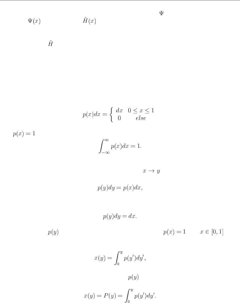
However, in most cases of interest we do not have the exact . But if we have made a clever

choice for

, the expression exhibits a smooth behavior in the neighbourhood of the

exact solution.

This means in turn that when do our Monte Carlo sampling, we will hopefully pick only

relevant values for .

The above example encompasses the main essence of the Monte Carlo philosophy. It is a

trial approach, where intelligent guesses lead to hopefully better results.

9.5.1 Change of variables

The starting point is always the uniform distribution

(9.68)

with

and satisfying

(9.69)

All random number generators provided in the program library generate numbers in this domain.

When we attempt a transformation to a new variable

we have to conserve the proba-

bility

(9.70)

which for the uniform distribution implies

(9.71)

Let us assume that

is a PDF different from the uniform PDF with . If we

integrate the last expression we arrive at

(9.72)

which is nothing but the cumulative distribution of

, i.e.,

(9.73)

This is an important result which has consequences for eventual improvements over the brute

force Monte Carlo.

To illustrate this approach, let us look at some examples.

152 CHAPTER 9. OUTLINE OF THE MONTE-CARLO STRATEGY

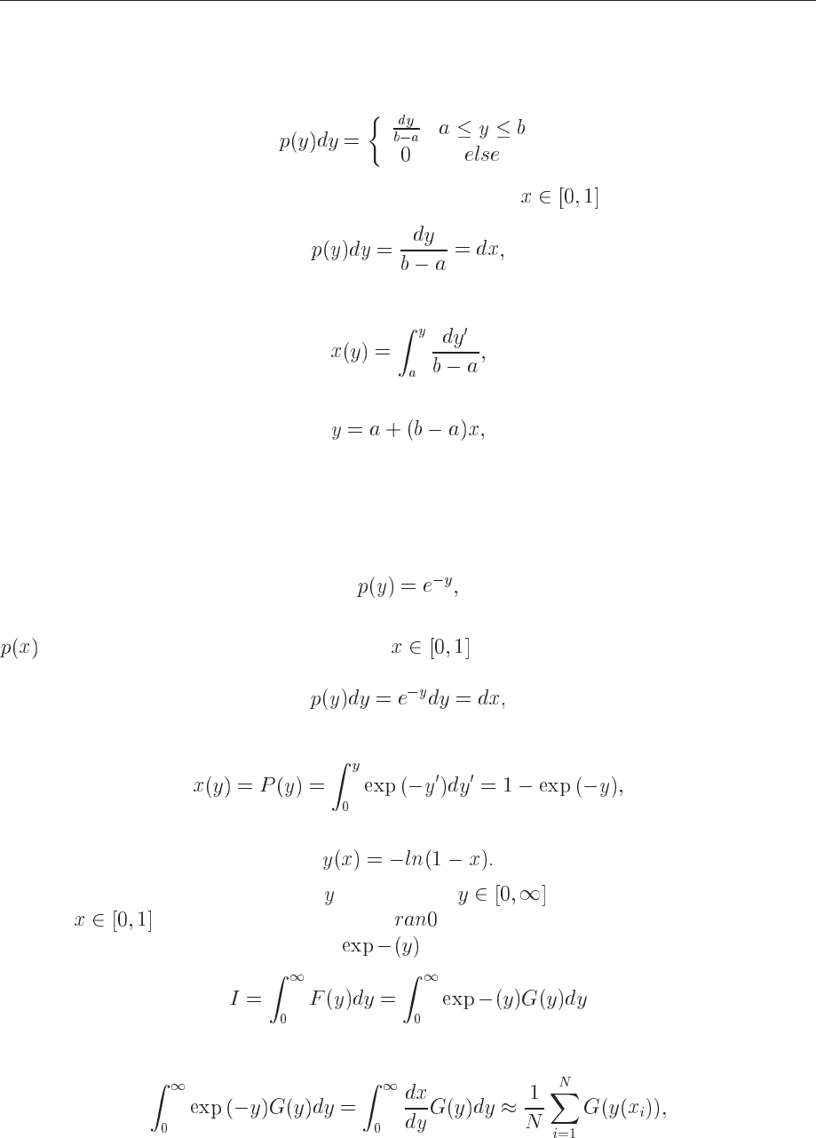
Example 1

Suppose we have the general uniform distribution

(9.74)

If we wish to relate this distribution to the one in the interval

we have

(9.75)

and integrating we obtain the cumulative function

(9.76)

yielding

(9.77)

a well-known result!

Example 2, the exponential distribution

Assume that

(9.78)

which is the exponential distribution, important for the analysis of e.g., radioactive decay. Again,

is given by the uniform distribution with , and with the assumption that the proba-

bility is conserved we have

(9.79)

which yields after integration

(9.80)

(9.81)

This gives us the new random variable in the domain determined through the random

variable generated by functions like .

This means that if we can factor out

from an integrand we may have

(9.82)

which we rewrite as

(9.83)

9.5. IMPROVED MONTE CARLO INTEGRATION 153

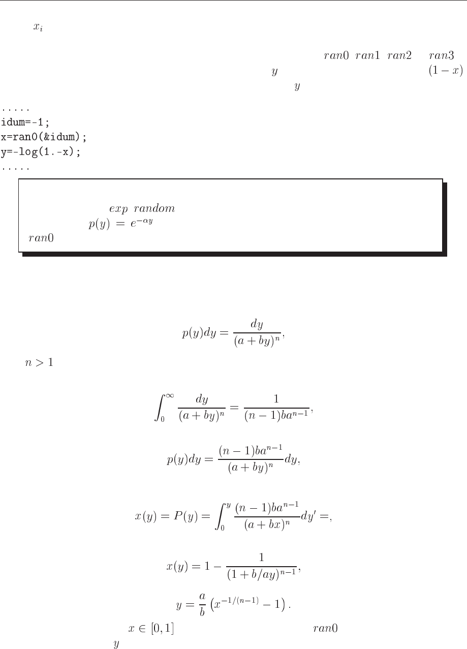
where is a random number in the interval [0,1].

The algorithm for the last example is rather simple. In the function which sets up the integral,

we simply need to call one of the random number generators like

, , or in

order to obtain numbers in the interval [0,1]. We obtain by the taking the logarithm of .

Our calling function which sets up the new random variable

may then include statements like

Exercise 9.4

Make a function _ which computes random numbersfor the exponential

distribution

based on random numbers generated from the function

Example 3

Another function which provides an example for a PDF is

(9.84)

with

. It is normalizable, positive deﬁnite, analytically integrable and the integral is invert-

ible, allowing thereby the expression of a new variable in terms of the old one. The integral

(9.85)

gives

(9.86)

which in turn gives the cumulative function

(9.87)

resulting in

(9.88)

(9.89)

With the random variable

generated by functions like , we have again the appro-

priate random variable for a new PDF.

154 CHAPTER 9. OUTLINE OF THE MONTE-CARLO STRATEGY

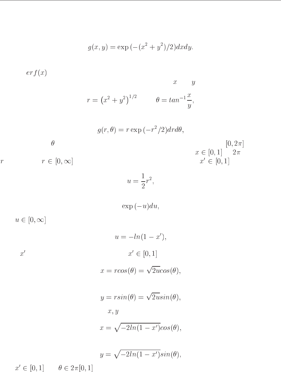
Example 4, the normal distribution

For the normal distribution, expressed here as

(9.90)

it is rather difﬁcult to ﬁnd an inverse since the cumulative distribution is given by the error

function

If we however switch to polar coordinates, we have for

and

(9.91)

resulting in

(9.92)

where the angle

could be given by a uniform distribution in the region . Following

example 1 above, this implies simply multiplying random numbers by . The variable

, deﬁned for needs to be related to to random numbers . To achieve that,

we introduce a new variable

(9.93)

and deﬁne a PDF

(9.94)

with

. Using the results from example 2, we have that

(9.95)

where

is a random number generated for . With

(9.96)

and

(9.97)

we can obtain new random numbers

through

(9.98)

and

(9.99)

with

and .

A function which yields such random numbers for the normal distribution would include

statements like

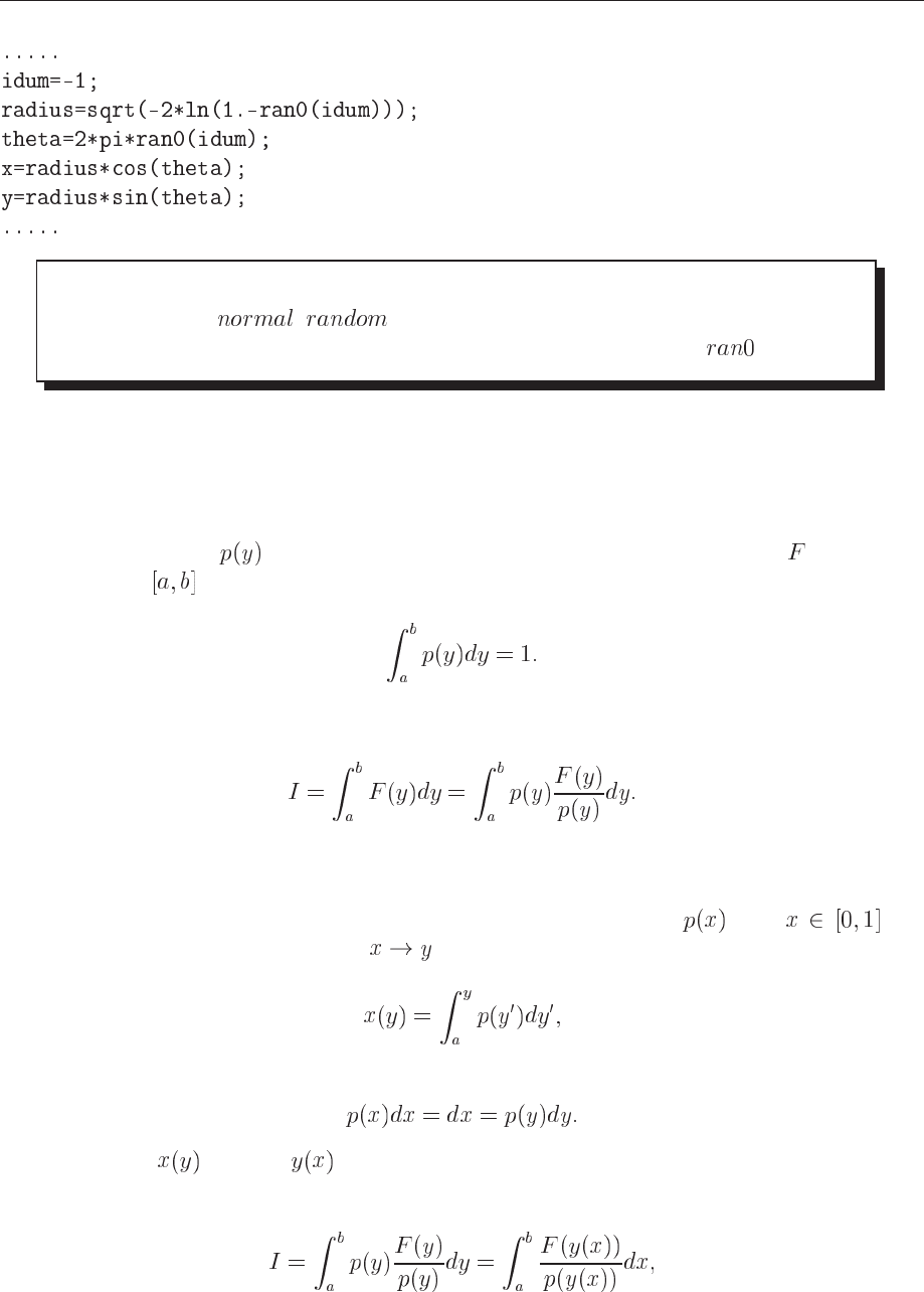
9.5. IMPROVED MONTE CARLO INTEGRATION 155

Exercise 9.4

Make a function _ whichcomputes random numbers for the normal

distribution based on random numbers generated from the function

9.5.2 Importance sampling

With the aid of the above variable transformations we address now one of the most widely used

approaches to Monte Carlo integration, namely importance sampling.

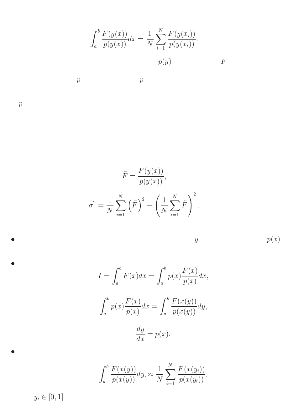
Let us assume that is a PDF whose behavior resembles that of a function deﬁned in a

certain interval

. The normalization condition is

(9.100)

We can rewrite our integral as

(9.101)

This integral resembles our discussion on the evaluation of the energy for a quantum mechanical

system in Eq. (9.64).

Since random numbers are generated for the uniform distribution

with , we

need to perform a change of variables through

(9.102)

where we used

(9.103)

If we can invert

, we ﬁnd as well.

With this change of variables we can express the integral of Eq. (9.101) as

(9.104)

156 CHAPTER 9. OUTLINE OF THE MONTE-CARLO STRATEGY

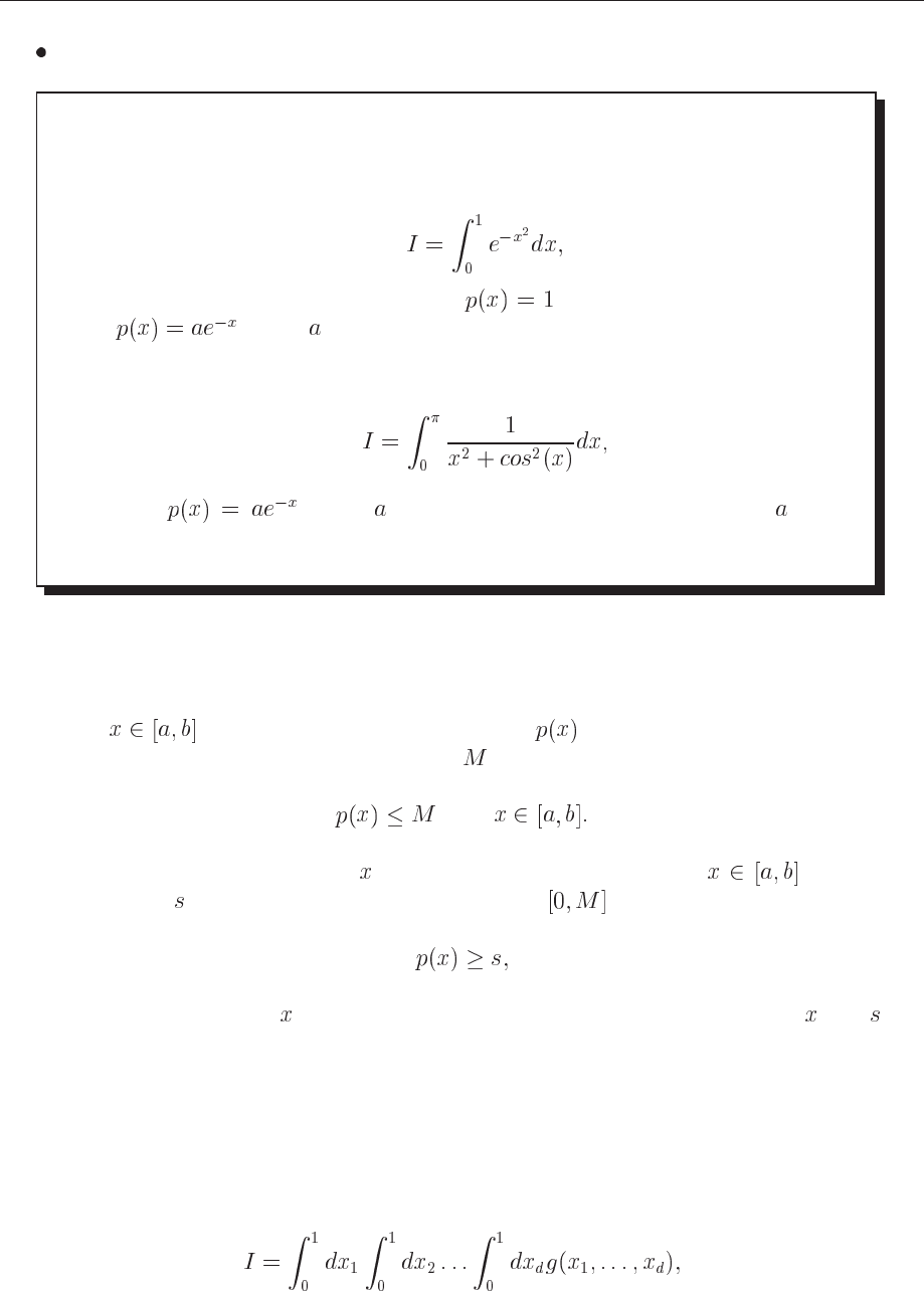
meaning that a Monte Carlo evalutaion of the above integral gives

(9.105)

The advantage of such a change of variables in case follows closely is that the integrand

becomes smooth and we can sample over relevant values for the integrand. It is however not triv-

ial to ﬁnd such a function

. The conditions on which allow us to perform these transformations

are

is normalizable and positive deﬁnite,

2. it is analytically integrable and

3. the integral is invertible, allowing us thereby to express a new variable in terms of the old

one.

The standard deviation is now with the deﬁnition

(9.106)

(9.107)

The algorithm for this procedure is

Use the uniform distribution to ﬁnd the random variable in the interval [0,1]. is

auser provided PDF.

Evaluate thereafter

(9.108)

by rewriting

(9.109)

since

(9.110)

Perform then a Monte Carlo sampling for

(9.111)

with ,

9.6. MONTE CARLO INTEGRATION OF MULTIDIMENSIONAL INTEGRALS 157

and evaluate the variance as well according to Eq. (9.107).

Exercise 9.5

(a) Calculate the integral

using brute force Monte Carlo with and importance sampling with

where is a constant.

(b) Calculate the integral

with where is a constant. Determine the value of which

minimizes the variance.

9.5.3 Acceptance-Rejection method

This is rather simple and appealing method after von Neumann. Assume that we are looking at

an interval

, this being the domain of the PDF . Suppose also that the largest value

our distribution function takes in this interval is , that is

(9.112)

Then we generate a random number

from the uniform distribution for and a corre-

sponding number for the uniform distribution between . If

(9.113)

we accept the new value of , else we generate again two new random numbers and and

perform the test in the latter equation again.

9.6 Monte Carlo integration of multidimensional integrals

When we deal with multidimensional integrals of the form

(9.114)

158 CHAPTER 9. OUTLINE OF THE MONTE-CARLO STRATEGY

with deﬁned in the interval we would typically need a transformation of variables of

the form

if we were to use the uniform distribution on the interval . In this case, we need a Jacobi

determinant

and to convert the function to

As an example, consider the following sixth-dimensional integral

(9.115)

where

(9.116)

with

We can solve this integral by employing our brute scheme, or using importance sampling and

random variables distributed according to a gaussian PDF. For the latter, if we set the mean value

and the standard deviation , we have

(9.117)

and through

(9.118)

we can rewrite our integral as

(9.119)

where is the gaussian distribution.

Below we list two codes, one for the brute force integration and the other employing impor-

tance sampling with a gaussian distribution.