Hirsch M., Smale S., Devaney R., Differential Equations, Dynamical Systems, and an Introduction to Chaos

Подождите немного. Документ загружается.

186 Chapter 8 Equilibria in Nonlinear Systems

6. Given an example of a family of differential equations x



= f

(x) for

which there are no equilibrium points if a<0; a single equilibrium if

a = 0; and four equilibrium points if a>0. Sketch the bifurcation

diagram for this family.

7. Discuss the local and global behavior of solutions of



= r − r



= sin

(θ) + a

at the bifurcation value a =−1.

8. Discuss the local and global behavior of solutions of



= r − r



= sin

(θ/2) + a

at all of the bifurcation values.

9. Consider the system



= r − r



= sin θ + a

(a) For which values of a does this system undergo a bifurcation?

(b) Describe the local behavior of solutions near the bifurcation values

(at, before, and after the bifurcation).

(d) Discuss any global changes that occur at the bifurcations.

10. Let X



= F (X) be a nonlinear system in R

. Suppose that F(0) = 0 and

that DF

has n distinct eigenvalues with negative real parts. Describe the

construction of a conjugacy between this system and its linearization.

11. Consider the system X



= F(X ) where X ∈ R

. Suppose that F has an

equilibrium point at X

. Show that there is a change of coordinates that

moves X

to the origin and converts the system to



= AX + G(X)

where A is an n × n matrix, which is the canonical form of DF

and

where G(X) satisﬁes

lim

|X|→0

|G(X)|

|X|

= 0.

Exercises 187

12. In the deﬁnition of an asymptotically stable equilibrium point, we

required that the equilibrium point also be stable. This requirement is

not vacuous. Give an example of a phase portrait (a sketch is sufﬁcient)

that has an equilibrium point toward which all nearby solution curves

(eventually) tend, but that is not stable.

This Page Intentionally Left Blank

Global Nonlinear Techniques

In this chapter we present a variety of qualitative techniques for analyzing

the behavior of nonlinear systems of differential equations. The reader should

be forewarned that none of these techniques works for all nonlinear systems;

most work only in specialized situations, which, as we shall see in the ensuing

chapters, nonetheless occur in many important applications of differential

equations.

9.1 Nullclines

One of the most useful tools for analyzing nonlinear systems of differential

equations (especially planar systems) are the nullclines. For a system in the

form



= f

,...,x

)



= f

,...,x

the x

-nullcline is the set of points where x



vanishes, so the x

-nullcline is the

set of points determined by setting f

, ..., x

) = 0.

The x

-nullclines usually separate R

into a collection of regions in which

the x

-components of the vector ﬁeld point in either the positive or negative

direction. If we determine all of the nullclines, then this allows us to decompose

189

190 Chapter 9 Global Nonlinear Techniques

into a collection of open sets, in each of which the vector ﬁeld points in a

“certain direction.”

This is easiest to understand in the case of a planar system



= f (x, y)



= g (x, y).

On the x-nullclines, we have x



= 0, so the vector ﬁeld points straight up

or down, and these are the only points at which this happens. Therefore the

x-nullclines divide

into regions where the vector ﬁeld points either to the

left or to the right. Similarly, on the y-nullclines, the vector ﬁeld is horizontal,

so the y-nullclines separate

into regions where the vector ﬁeld points either

upward or downward. The intersections of the x- and y-nullclines yield the

equilibrium points. In any of the regions between the nullclines, the vector ﬁeld

is neither vertical nor horizontal, so it must point in one of four directions:

northeast, northwest, southeast, or southwest. We call such regions basic

regions. Often, a simple sketch of the basic regions allows us to understand the

phase portrait completely, at least from a qualitative point of view.

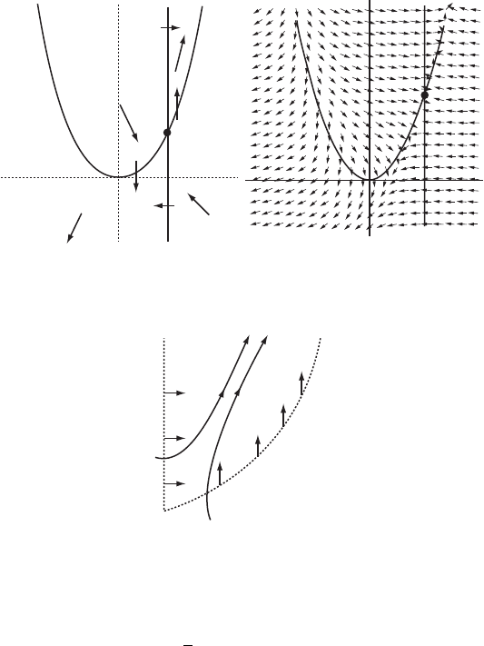
Example. For the system



= y − x



= x − 2,

the x-nullcline is the parabola y = x

and the y-nullcline is the vertical line x =

2. These nullclines meet at (2, 4) so this is the only equilibrium point. The null-

clines divide

into four basic regions labeled A through D in Figure 9.1(a).

By ﬁrst choosing one point in each of these regions, and then determining the

direction of the vector ﬁeld at that point, we can decide the direction of the

vector ﬁeld at all points in the basic region. For example, the point (0, 1) lies in

region A and the vector ﬁeld is (1, −2) at this point, which points toward the

southeast. Hence the vector ﬁeld points southeast at all points in this region.

Of course, the vector ﬁeld may be nearly horizontal or nearly vertical in this

region; when we say southeast we mean that the angle θ of the vector ﬁeld lies

in the sector −π/2 < θ < 0. Continuing in this fashion we get the direction

of the vector ﬁeld in all four regions, as in Figure 9.1(b). This also determines

the horizontal and vertical directions of the vector ﬁeld on the nullclines.

Just from the direction ﬁeld alone, it appears that the equilibrium point is a

saddle. Indeed, this is the case because the linearized system at (2, 4) is





−41



9.1 Nullclines 191

(a)

(b)

Figure 9.1 The (a) nullclines and (b) direction field.

y⫽x

x⫽2

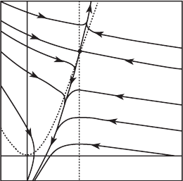
Figure 9.2 Solutions

enter the basic region

B and then tend to ∞.

which has eigenvalues −2 ±

√

5, one of which is positive, the other negative.

More importantly, we can ﬁll in the approximate behavior of solutions

everywhere in the plane. For example, note that the vector ﬁeld points into the

basic region marked B at all points along its boundary, and then it points north-

easterly at all points inside B. Thus any solution in region B must stay in region

B for all time and tend toward ∞ in the northeast direction. See Figure 9.2.

Similarly, solutions in the basic region D stay in that region and head toward

∞ in the southwest direction. Solutions starting in the basic regions A and

C have a choice: They must eventually cross one of the nullclines and enter

regions B and D (and therefore we know their ultimate behavior) or else they

tend to the equilibrium point. However, there is only one curve of such solu-

tions in each region, the stable curve at (2, 4). Thus we completely understand

the phase portrait for this system, at least from a qualitative point of view. See

Figure 9.3.



192 Chapter 9 Global Nonlinear Techniques

Figure 9.3 The nullclines and

phase portrait for x



= y−x



= x − 2.

Example. (Heteroclinic Bifurcation) Next consider the system that

depends on a parameter a:



= x

− 1



=−xy + a(x

− 1).

The x-nullclines are given by x =±1 while the y-nullclines are xy = a(x

−1).

The equilibrium points are (±1, 0). Since x



= 0onx ± 1, the vector ﬁeld is

actually tangent to these nullclines. Moreover, we have y



=−y on x = 1 and



= y on x =−1. So solutions tend to (1, 0) along the vertical line x = 1 and

tend away from (−1, 0) along x =−1. This happens for all values of a.

Now, let’s look at the case a = 0. Here the system simpliﬁes to



= x

− 1



=−xy,

so y



= 0 along the axes. In particular, the vector ﬁeld is tangent to the x-axis

and is given by x



= x

− 1 on this line. So we have x



> 0if|x| > 1 and



< 0if|x| < 1. Thus, at each equilibrium point, we have one straight-line

solution tending to the equilibrium and one tending away. So it appears that

each equilibrium is a saddle. This is indeed the case, as is easily checked by

linearization.

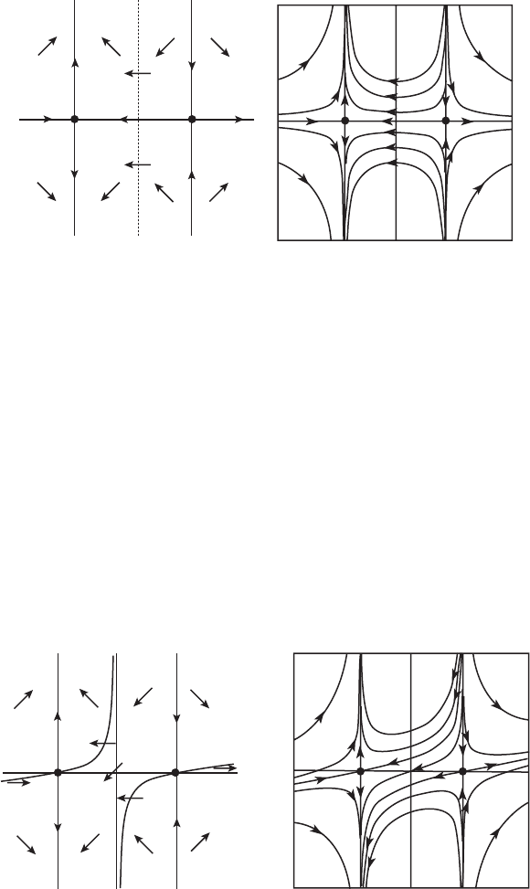
There is a second y-nullcline along x = 0, but the vector ﬁeld is not tangent

to this nullcline. Computing the direction of the vector ﬁeld in each of the

basic regions determined by the nullclines yields Figure 9.4, from which we

can deduce immediately the qualitative behavior of all solutions.

Note that, when a = 0, one branch of the unstable curve through (1, 0)

matches up exactly with a branch of the stable curve at (−1, 0). All solutions

9.1 Nullclines 193

(a)

(b)

Figure 9.4 The (a) nullclines and (b) phase portrait for x



− 1, y



= −xy.

on this curve simply travel from one saddle to the other. Such solutions are

called heteroclinic solutions or saddle connections. Typically, for planar systems,

stable and unstable curves rarely meet to form such heteroclinic “connections.”

When they do, however, one can expect a bifurcation.

Now consider the case where a = 0. The x-nullclines remain the same, at

x =±1. But the y-nullclines change drastically as shown in Figure 9.5. They

are given by y = a(x

− 1)/x.

When a>0, consider the basic region denoted by A. Here the vector ﬁeld

points southwesterly. In particular, the vector ﬁeld points in this direction

along the x-axis between x =−1 and x = 1. This breaks the heteroclinic

connection: The right portion of the stable curve associated to (−1, 0) must

(a)

(b)

Figure 9.5 The (a) nullclines and (b) phase plane when a > 0 after

the heteroclinic bifurcation.

194 Chapter 9 Global Nonlinear Techniques

now come from y =∞in the upper half plane, while the left portion of the

unstable curve associated to (1, 0) now descends to y =−∞in the lower

half plane. This opens an “avenue” for certain solutions to travel from y =

+∞ to y =−∞between the two lines x =±1. Whereas when a = 0 all

solutions remain for all time conﬁned to either the upper or lower half-plane,

the heteroclinic bifurcation at a = 0 opens the door for certain solutions to

make this transit.

A similar situation occurs when a<0 (see Exercise 2 at the end of this

chapter).



9.2 Stability of Equilibria

Determining the stability of an equilibrium point is straightforward if the

equilibrium is hyperbolic. When this is not the case, this determination

becomes more problematic. In this section we develop an alternative method

for showing that an equilibrium is asymptotically stable. Due to the Russian

mathematician Liapunov, this method generalizes the notion that, for a linear

system in canonical form, the radial component r decreases along solution

curves. Liapunov noted that other functions besides r could be used for this

purpose. Perhaps more importantly, Liapunov’s method gives us a grasp on

the size of the basin of attraction of an asymptotically stable equilibrium point.

By deﬁnition, the basin of attraction is the set of all initial conditions whose

solutions tend to the equilibrium point.

Let L :

O → R be a differentiable function deﬁned on an open set O in R

that contains an equilibrium point X

∗

of the system X



= F(X). Consider the

function

L(X ) = DL

(F(X )).

As we have seen, if φ

(X) is the solution of the system passing through X when

t = 0, then we have

L(X ) =



t=0

L ◦ φ

(X)

by the chain rule. Consequently, if

L(X ) is negative, then L decreases along

the solution curve through X .

We can now state Liapunov’s stability theorem:

Theorem. (Liapunov Stability) Let X

∗

be an equilibrium point for X



F(X ). Let L :

O → R be a differentiable function deﬁned on an open set O

9.2 Stability of Equilibria 195

containing X

∗

. Suppose further that

(a) L(X

∗

) = 0 and L(X) > 0 if X = X

∗

;

(b)

L ≤ 0 in

O − X

∗

Then X

∗

is stable. Furthermore, if L also satisﬁes

(c)

L<0 in

O − X

∗

then X

∗

is asymptotically stable. 

A function L satisfying (a) and (b) is called a Liapunov function for X

∗

.If

Note that Liapunov’s theorem can be applied without solving the differential

equation; all we need to compute is DL

(F(X )). This is a real plus! On the

other hand, there is no cut-and-dried method of ﬁnding Liapunov functions; it

is usually a matter of ingenuity or trial and error in each case. Sometimes there

are natural functions to try. For example, in the case of mechanical or electrical

systems, energy is often a Liapunov function, as we shall see in Chapter 13.

Example. Consider the system of differential equations in

given by



= (x + 2y)(z + 1)



= (−x + y)(z + 1)



=−z

where  is a parameter. The origin is the only equilibrium point for this system.

The linearization of the system at (0, 0, 0) is



⎛

⎝

 20

−1  0

000

⎞

⎠

Y .

The eigenvalues are 0 and  ±

√

2i. Hence, from the linearization, we can only

conclude that the origin is unstable if  > 0. When  ≤ 0, all we can conclude

is that the origin is not hyperbolic.

When  ≤ 0 we search for a Liapunov function for (0, 0, 0) of the form

L(x, y, z) = ax

+ by

+ cz

, with a, b, c>0. For such an L, we have

L = 2(axx



+ byy



+ czz



so that

L/2 = ax(x + 2y)(z + 1) + by(−x + y)(z + 1) − cz

= (ax

+ by

)(z + 1) + (2a − b)(xy)(z + 1) − cz