Hirsch M., Smale S., Devaney R., Differential Equations, Dynamical Systems, and an Introduction to Chaos

Подождите немного. Документ загружается.

196 Chapter 9 Global Nonlinear Techniques

For stability, we want

L ≤ 0; this can be arranged, for example, by setting

a = 1, b = 2, and c = 1. If  = 0, we then have

L =−z

≤ 0, so the origin

is stable. It can be shown (see Exercise 4) that the origin is not asymptotically

stable in this case.

If  < 0, then we ﬁnd

L = (x

+ 2y

)(z + 1) − z

so that

L<0 in the region O given by z>−1 (minus the origin). We conclude

that the origin is asymptotically stable in this case, and, indeed, from Exercise 4,

that all solutions that start in the region

O tend to the origin. 

Example. (The Nonlinear Pendulum) Consider a pendulum consisting

of a light rod of length  to which is attached a ball of mass m. The other end

of the rod is attached to a wall at a point so that the ball of the pendulum

moves on a circle centered at this point. The position of the mass at time t

is completely described by the angle θ(t ) of the mass from the straight down

position and measured in the counterclockwise direction. Thus the position

of the mass at time t is given by ( sin θ(t ), − cos θ(t )).

The speed of the mass is the length of the velocity vector, which is  dθ/dt ,

and the acceleration is  d

θ/dt

. We assume that the only two forces acting

on the pendulum are the force of gravity and a force due to friction. The

gravitational force is a constant force equal to mg acting in the downward

direction; the component of this force tangent to the circle of motion is given

by −mg sin θ . We take the force due to friction to be proportional to velocity

and so this force is given by −b dθ/dt for some constant b>0. When there

is no force due to friction (b = 0), we have an ideal pendulum. Newton’s law

then gives the second-order differential equation for the pendulum

m

=−b

dθ

− mg sin θ.

For simplicity, we assume that units have been chosen so that m =  = g = 1.

Rewriting this equation as a system, we introduce v = dθ/dt and get



= v



=−bv − sin θ.

Clearly, we have two equilibrium points (mod 2π ): the downward rest position

at θ = 0, v = 0, and the straight-up position θ = π, v = 0. This upward

postion is an unstable equilibrium, both from a mathematical (check the

linearization) and physical point of view.

9.2 Stability of Equilibria 197

For the downward equilibrium point, the linearized system is





−1 −b



Y .

The eigenvalues here are either pure imaginary (when b = 0) or else have neg-

ative real parts (when b>0). So the downward equilibrium is asymptotically

stable if b>0 as everyone on earth who has watched a real-life pendulum

knows.

To investigate this equilibrium point further, consider the function

E(θ , v) =

+ 1 − cos θ. For readers with a background in elementary

mechanics, this is the well-known total energy function, which we will describe

further in Chapter 13. We compute

E = vv



+ sin θθ



=−bv

so that

E ≤ 0. Hence E is a Liapunov function. Thus the origin is a stable

equilibrium. If b = 0 (that is, there is no friction), then

E ≡ 0. That is, E is

constant along all solutions of the system. Hence we may simply plot the level

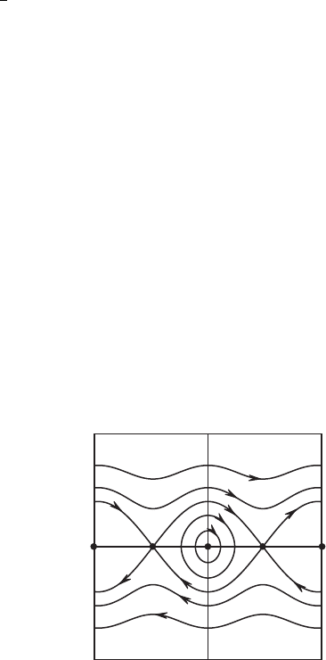
curves of E to see where the solution curves reside. We ﬁnd the phase portrait

shown in Figure 9.6. Note that we do not have to solve the differential equation

to paint this picture; knowing the level curves of E (and the direction of the

vector ﬁeld) tells us everything. We will encounter many such (very special)

functions that are constant along solution curves later in this chapter.

The solutions encircling the origin have the property that −π < θ (t) < π

for all t . Therefore these solutions correspond to the pendulum oscillating

about the downward rest position without ever crossing the upward position

θ = π . The special solutions connecting the equilibrium points at (±π ,0)

2π⫺2π

Figure 9.6 The phase portrait for the

ideal pendulum.

198 Chapter 9 Global Nonlinear Techniques

correspond to the pendulum tending to the upward-pointing equilibrium in

both the forward and backward time directions. (You don’t often see such

motions!) Beyond these special solutions we ﬁnd solutions for which θ (t)

either increases or decreases for all time; in these cases the pendulum spins

forever in the counterclockwise or clockwise direction.



We will return to the pendulum example for the case b>0 later, but ﬁrst

we prove Liapunov’s theorem.

Proof: Let δ > 0 be so small that the closed ball B

∗

) around the equilib-

rium point X

∗

of radius δ lies entirely in O. Let α be the minimum value of

L on the boundary of B

∗

), that is, on the sphere S

∗

) of radius δ and

center X

∗

. Then α > 0 by assumption. Let U ={X ∈ B

∗

) | L(X ) < α}

and note that X

∗

lies in U. Then no solution starting in U can meet S

∗

)

since L is nonincreasing on solution curves. Hence every solution starting

U never leaves B

∗

). This proves that X

∗

is stable.

Now suppose that assumption (c) in the Liapunov stability theorem holds

as well, so that L is strictly decreasing on solutions in

U − X

∗

. Let X (t )be

a solution starting in

U − X

∗

and suppose that X (t

) → Z

∈ B

∗

) for

some sequence t

→∞. We claim that Z

= X

∗

. To see this, observe that

L(X (t )) >L(Z

) for all t ≥ 0 since L(X (t)) decreases and L(X (t

)) → L(Z

)

by continuity of L.IfZ

= X

∗

, let Z (t ) be the solution starting at Z

. For

any s>0, we have L(Z (s)) <L(Z

). Hence for any solution Y (s) starting

sufﬁciently near Z

we have

L(Y (s)) <L

(

)

Setting Y (0) = X(t

) for sufﬁciently large n yields the contradiction

L(X

(

+ s

)

) <L

(

)

Therefore Z

= X

∗

. This proves that X

∗

is the only possible limit point of the

set {X (t ) | t ≥ 0} and completes the proof of Liapunov’s theorem.



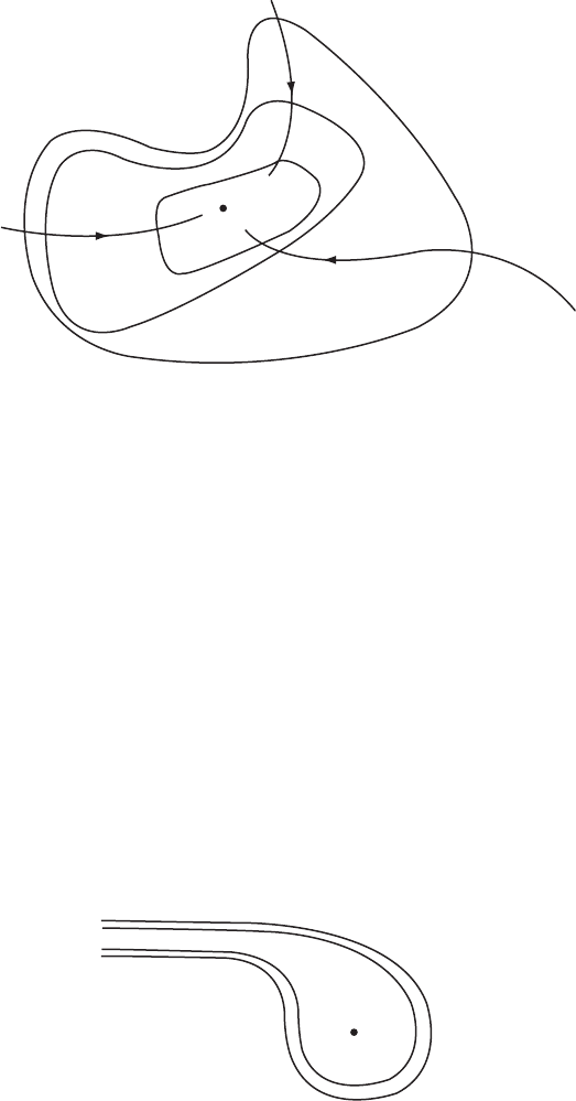
Figure 9.7 makes the theorem intuitively obvious. The condition

L<0

means that when a solution crosses a “level surface” L

−1

(c), it moves inside

the set where L ≤ c and can never come out again. Unfortunately, it is

sometimes difﬁcult to justify the diagram shown in this ﬁgure; why should the

sets L

−1

∗

? Of course, in many cases, Figure 9.7 is indeed

correct, as, for example, if L is a quadratic function such as ax

+ by

with

a, b>0. But what if the level surfaces look like those shown in Figure 9.8? It

is hard to imagine such an L that fulﬁlls all the requirements of a Liapunov

function; but rather than trying to rule out that possibility, it is simpler to give

the analytic proof as above.

9.2 Stability of Equilibria 199

⫺1

)

⫺1

)

⫺1

)

Figure 9.7 Solutions decrease through the level sets L

−1

)

of a strict Liapunov function.

Example. Now consider the system



=−x



=−y(x

+ z

+ 1)



=−sin z.

The origin is again an equilibrium point. It is not the only one, however,

since (0, 0, nπ ) is also an equilibrium point for each n ∈

Z. Hence the origin

cannot be globally asymptotically stable. Moreover, the planes z = nπ for

n ∈

Z are invariant in the sense that any solution that starts on one of these

planes remains there for all time. This occurs since z



= 0 when z = nπ.In

particular, any solution that begins in the region |z| < π must remain trapped

in this region for all time.

⫺1

)

⫺1

)

Figure 9.8 Level sets of a Liapunov

function may look like this.

200 Chapter 9 Global Nonlinear Techniques

Linearization at the origin yields the system



⎛

⎝

000

0 −10

00−1

⎞

⎠

which tells us nothing about the stability of this equilibrium point.

However, consider the function

L(x, y, z) = x

+ y

+ z

Clearly, L>0 except at the origin. We compute

L =−2x

− 2y

+ z

+ 1) − 2z sin z.

Then

L<0 at all points in the set |z| < π (except the origin) since z sin z>0

when z = 0. Hence the origin is asymptotically stable.

Moreover, we can conclude that the basin of attraction of the origin is the

entire region |z| < π. From the proof of the Liapunov stability theorem, it

follows immediately that any solution that starts inside a sphere of radius r<π

must tend to the origin. Outside of the sphere of radius π and between the

planes z =±π, the function L is still strictly decreasing. Since solutions are

trapped between these two planes, it follows that they too must tend to the

origin.



Liapunov functions not only detect stable equilibria; they can also be used to

estimate the size of the basin of attraction of an asymptotically stable equilib-

rium, as the above example shows. The following theorem gives a criterion for

asymptotic stability and the size of the basin even when the Liapunov function

is not strict. To state it, we need several deﬁnitions.

Recall that a set

P is called invariant if for each X ∈ P, φ

(X) is deﬁned

and in

P for all t ∈ R. For example, the region |z| < π in the above example

is an invariant set. The set

P is positively invariant if for each X ∈ P, φ

(X)

is deﬁned and in

P for all t ≥ 0. The portion of the region |z| < π inside

a sphere centered at the origin in the previous example is positively invariant

but not invariant. Finally, an entire solution of a system is a set of the form

{

(X) | t ∈ R

}

Theorem. (Lasalle’s Invariance Principle) Let X

∗

be an equilibrium

point for X



= F(X ) and let L : U → R be a Liapunov function for X

∗

, where

U is an open set containing X

∗

. Let P ⊂ U be a neighborhood of X

∗

that is closed

and bounded. Suppose that

P is positively invariant, and that there is no entire

solution in

P −X

∗

on which L is constant. Then X

∗

is asymptotically stable, and

P is contained in the basin of attraction of X

∗

. 

9.2 Stability of Equilibria 201

Before proving this theorem we apply it to the equilibrium X

∗

= (0, 0) of

the damped pendulum discussed previously. Recall that a Liapunov function

is given by E(θ , v) =

+ 1 − cos θ and that

E =−bv

. Since

E = 0on

v = 0, this Liapunov function is not strict.

To estimate the basin of (0, 0), ﬁx a number c with 0 <c<2, and deﬁne

={(θ, v) | E(θ , v) ≤ c and |θ | < π }.

Clearly, (0, 0) ∈

. We shall prove that P

lies in the basin of attraction of

(0, 0).

Note ﬁrst that

is positively invariant. To see this suppose that (θ(t ), v(t ))

is a solution with (θ(0), v(0)) ∈

. We claim that (θ(t ), v(t )) ∈ P

for all

t ≥ 0. We clearly have E(θ (t), v(t)) ≤ c since

E ≤ 0. If |θ(t )|≥π, then there

must exist a smallest t

such that θ (t

) =±π. But then

E(θ (t

), v(t

)) = E(±π, v(t

))

v(t

)

+ 2

≥ 2.

However,

E(θ (t

), v(t

)) ≤ c<2.

This contradiction shows that θ (t

) < π , and so P

is positively invariant.

We now show that there is no entire solution in

on which E is constant

(except the equilibrium solution). Suppose there is such a solution. Then,

along that solution,

E ≡ 0 and so v ≡ 0. Hence, θ



= 0soθ is constant on

the solution. We also have v



=−sin θ = 0 on the solution. Since |θ | < π ,it

follows that θ ≡ 0. Thus the only entire solution in

on which E is constant

is the equilibrium point (0, 0).

Finally,

is a closed set. Because if (θ

, v

) is a limit point of P

, then |θ

|≤

π, and E(θ

, v

) ≤ c by continuity of E. But |θ

|=π implies E(θ

, v

) >c,

as shown above. Hence |θ

| < π and so (θ

, v

) does belong to P

,soP

closed.

From the theorem we conclude that

belongs to the basin of attraction of

(0, 0) for each c<2; hence the set

P =∪

{

| 0 <c<2

}

is also contained in this basin. Note that we may write

P ={(θ, v) | E(θ , v) < 2 and |θ| < π }.

202 Chapter 9 Global Nonlinear Techniques

᎐o

Figure 9.9 The curve γ

bounds the region P

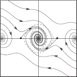
Figure 9.9 displays the phase portrait for the damped pendulum. The curves

marked γ

are the level sets E(θ, v) = c. Note that solutions cross each of these

curves exactly once and eventually tend to the origin.

This result is quite natural on physical grounds. For if θ =±π, then

E(θ ,0) < 2 and so the solution through (θ , 0) tends to (0, 0). That is, if

we start the pendulum from rest at any angle θ except the vertical position,

the pendulum will eventually wind down to rest at its stable equilibrium

postion.

There are other initial positions in the basin of (0, 0) that are not in the set

P. For example, consider the solution through (−π, u), where u is very small

but not zero. Then (−π, u) ∈

P, but the solution through this point moves

quickly into

P, and therefore eventually approaches (0, 0). Hence (−π , u) also

lies in the basin of attraction of (0, 0). This can be seen in Figure 9.9, where the

solutions that begin just above the equilibrium point at (−π , 0) and just below

(π, 0) quickly cross γ

and then enter P

. See Exercise 5 for further examples

of this.

We now prove the theorem.

Proof: Imagine a solution X(t ) that lies in the positively invariant set

P for

0 ≤ t ≤∞, but suppose that X(t ) does not tend to X

∗

as t →∞. Since P

is closed and bounded, there must be a point Z = X

∗

in P and a sequence

→∞such that

lim

n→∞

X(t

) = Z .

We may assume that the sequence {t

} is an increasing sequence.

We claim that the entire solution through Z lies in

P. That is, φ

(Z)is

deﬁned and in

P for all t ∈ R, not just t ≥ 0. This can be seen as follows.

9.3 Gradient Systems 203

First, φ

(Z) is certainly deﬁned for all t ≥ 0 since P is positively invariant. On

the other hand, φ

(X(t

)) is deﬁned and in P for all t in the interval [−t

,0].

Since {t

} is an increasing sequence, we have that φ

(X(t

n+k

)) is also deﬁned

and in

P for all t ∈[−t

,0] and all k ≥ 0. Since the points X (t

n+k

) → Z

as k →∞, it follows from continuous dependence of solutions on initial

conditions that φ

(Z) is deﬁned and in P for all t ∈[−t

,0]. Since this

holds for any t

, we see that the solution through Z is an entire solution lying

Finally, we show that L is constant on the entire solution through Z .If

L(Z ) = α, then we have L(X (t

)) ≥ α and moreover

lim

n→∞

L(X (t

)) = α.

More generally, if {s

}is any sequence of times for which s

→∞as n →∞,

then L(X(s

)) → α as well. This follows from the fact that L is nonincreas-

ing along solutions. Now the sequence X(t

+ s) converges to φ

(Z), and

so L(φ

(Z)) = α. This contradicts our assumption that there are no entire

solutions lying in

P on which L is constant and proves the theorem. 

In this proof we encountered certain points that were limits of a sequence

of points on the solution through X. The set of all points that are limit points

of a given solution is called the set of ω-limit points, or the ω-limit set, of the

solution X (t). Similarly, we deﬁne the set of α-limit points, or the α-limit set,

of a solution X(t ) to be the set of all points Z such that lim

n→∞

X(t

) = Z

for some sequence t

→−∞. (The reason, such as it is, for this terminol-

ogy is that α is the ﬁrst letter and ω the last letter of the Greek alphabet.)

The following facts, essentially proved above, will be used in the following

chapter.

Proposition. The α-limit set and the ω-limit set of a solution that is deﬁned

for all t ∈

R are closed, invariant sets. 

9.3 Gradient Systems

Now we turn to a particular type of system for which the previous material

on Liapunov functions is particularly germane. A gradient system on

is a

system of differential equations of the form



=−grad V (X )

204 Chapter 9 Global Nonlinear Techniques

where V : R

→ R is a C

∞

function, and

grad V =



∂V

∂x

, ...,

∂V

∂x



(The negative sign in this system is traditional.) The vector ﬁeld grad V is

called the gradient of V . Note that −grad V (X) = grad (−V (X )).

Gradient systems have special properties that make their ﬂows rather simple.

The following equality is fundamental:

(Y ) = grad V (X ) · Y .

This says that the derivative of V at X evaluated at Y = (y

, ..., y

) ∈ R

is given by the dot product of the vectors grad V (X ) and Y . This follows

immediately from the formula

(Y ) =



j=1

∂V

∂x

(X) y

Let X(t ) be a solution of the gradient system with X(0) = X

, and let

V :

→ R be the derivative of V along this solution. That is,

V (X) =

V (X(t )).

Proposition. The function V is a Liapunov function for the system X



−grad V (X). Moreover,

V (X) = 0 if and only if X is an equilibrium point.

Proof: By the chain rule we have

V (X) = DV



)

= grad V (X ) · (−grad V (X ))

=−|grad V (X )|

≤ 0.

In particular,

V (X) = 0 if and only if grad V (X ) = 0.



An immediate consequence of this is the fact that if X

∗

is an isolated mini-

mum of V , then X

∗

is an asymptotically stable equilibrium of the gradient

system. Indeed, the fact that X

∗

is isolated guarantees that

V<0ina

neighborhood of X

∗

(not including X

∗

To understand a gradient ﬂow geometrically we look at the level surfaces

of the function V :

→ R. These are the subsets V

−1

9.3 Gradient Systems 205

X ∈ V

−1

(c)isaregular point, that is, grad V (X) = 0, then V

−1

a “surface” of dimension n − 1 near X. To see this, assume (by renumbering

the coordinates) that ∂V /∂x

(X) = 0. Using the implicit function theorem,

we ﬁnd a C

∞

function g : R

n−1

→ R such that, near X, the level set V

−1

(c)

is given by



, ..., x

n−1

, g

(

, ..., x

n−1

)



= c.

That is, near X, V

−1

case where n = 2, V

−1

point. If all points in V

−1

value for V . In the case n = 2, if c is a regular value, then the level set V

−1

(c)

is a union of simple (or nonintersecting) curves. If X is a nonregular point for

V , then grad V (X) = 0, so X is a critical point for the function V , since all

partial derivatives of V vanish at X .

Now suppose that Y is a vector that is tangent to the level surface V

−1

(c)at

X. Then we can ﬁnd a curve γ (t ) in this level set for which γ



(0) = Y . Since

V is constant along γ , it follows that

(Y ) =



t=0

V ◦ γ (t ) = 0.

We thus have, by our observations above, that grad V (X) · Y = 0, or, in

other words, grad V (X ) is perpendicular to every tangent vector to the level

set V

−1

(c)atX. That is, the vector ﬁeld grad V (X ) is perpendicular to the

level surfaces V

−1

in the following theorem.

Theorem. (Properties of Gradient Systems) For the system X



−grad V (X ):

1. If c is a regular value of V , then the vector ﬁeld is perpendicular to the level

set V

−1

(c).

2. The critical points of V are the equilibrium points of the system.

3. If a critical point is an isolated minimum of V , then this point is an

asymptotically stable equilibrium point.



Example. Let V : R

→ R be the function V (x, y) = x

(x −1)

. Then

the gradient system



= F(X) =−grad V (X)

is given by



=−2x(x − 1)(2x − 1)



=−2y.