Heiman G. Basic Statistics for the Behavioral Sciences

Подождите немного. Документ загружается.

198 CHAPTER 9 / Using Probability to Make Decisions about Data

means almost never occur with this population. Therefore, if we do get such a mean,

we probably are not representing this population: We reject that the sample repre-

sents the underlying raw score population and decide that it represents some other

population.

Conversely, if our sample mean is not in the region of rejection, then the sample is

not unlikely to be representing the ordinary SAT population. In fact, by our definition,

samples not in the region of rejection are likely to represent this population, although

with some sampling error. In such cases, we retain the idea that the sample is simply

poorly representing this population of SAT scores.

How do we know where to draw the line that starts the region of rejection? By defin-

ing our criterion probability. The criterion probability is the probability that defines

samples as too unlikely for us to accept as representing a particular population.

Researchers usually use .05 as their default criterion probability. By this criterion, those

sample means that together would occur only 5% of the time when representing the

ordinary SAT population are so unlikely that if we get any one of them, we’ll reject that

our sample represents this population.

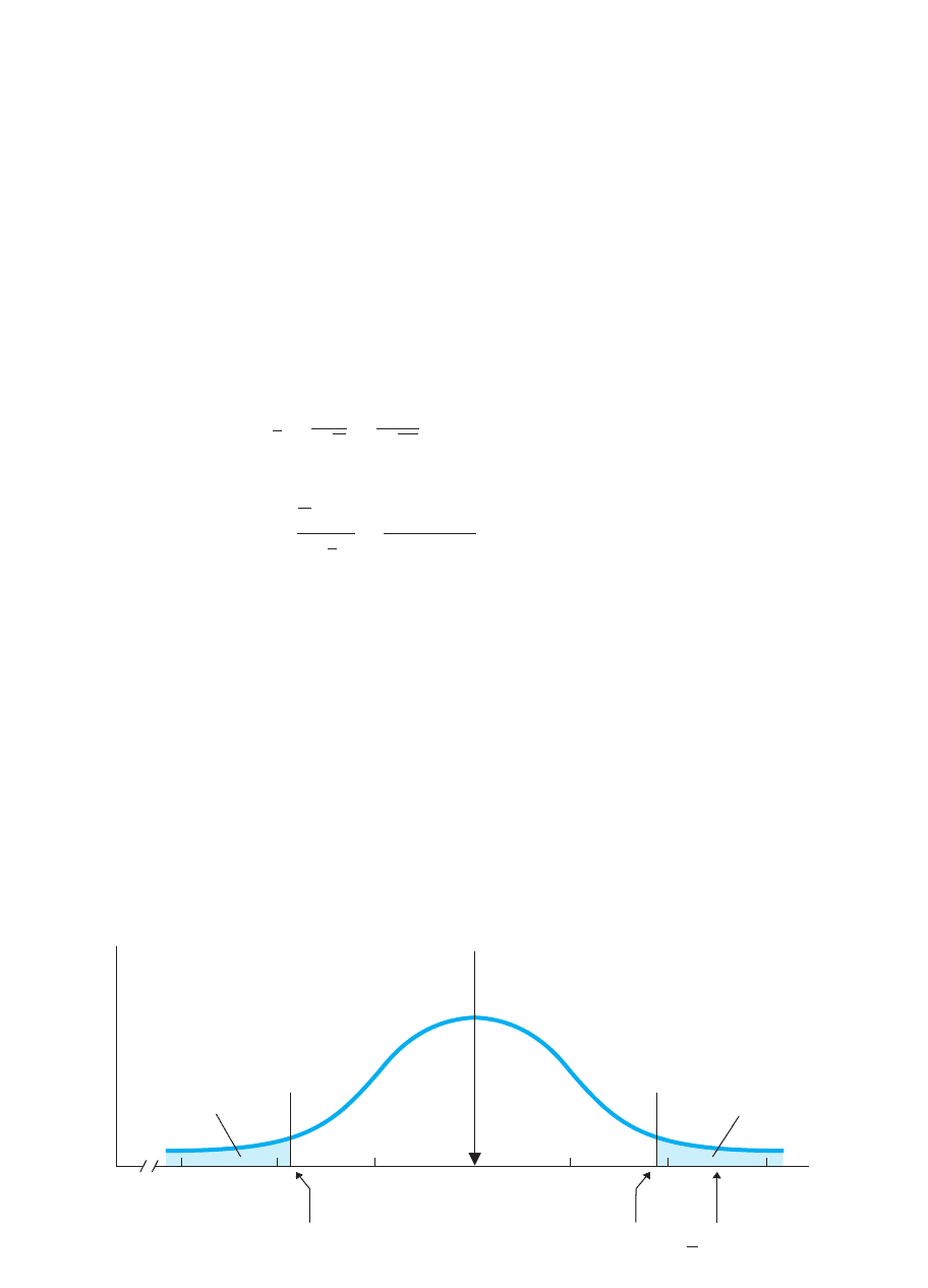
The criterion that we select determines the size of the region of rejection. The sam-

ple means that occur 5% of the time are those that make up the extreme 5% of the sam-

pling distribution. However, we consider the means that are above or below 500 that

together are a total of 5% of the curve, so we divide the 5% in half. Therefore, as

Figure 9.4 showed, the extreme 2.5% of the curve in each tail of the sampling distribu-

tion forms our region of rejection.

REMEMBER The criterion probability that defines samples as unlikely—and

also determines the size of the region of rejection—is usually

Now the task is simply to determine if our sample mean falls into the region of rejec-

tion. To do this, we will compare the sample’s z-score to the critical value.

Identifying the Critical Value

Figure 9.4 also showed our critical values. These are the z-scores at the lines that mark

the beginning of the upper and lower regions of rejection. Because z-scores get larger

as we go farther into the tails, if the z-score for our sample mean is greater than the crit-

ical value, then we know that our sample mean lies in the region of rejection. Thus, a

critical value marks the inner edge of the region of rejection and therefore defines the

value required for a sample to fall into the region of rejection. Essentially, it is the

minimum z-score that defines a sample as too unlikely.

REMEMBER The critical value of defines the minimum value of a sample

must have in order to be in the region of rejection.

How do we determine the critical value? By considering our criterion. With a

criterion of .05, we set up the region of rejection in Figure 9.4 so that in each tail is

the extreme 2.5%, or .025, of the total area under the curve. Then from the z-table in

Appendix C, we see that .025 of the curve lies beyond the z-score of 1.96. There-

fore, in each tail, the region of rejection begins at 1.96, so is our critical value

Thus, back in Figure 9.4, labeling the inner edges of the region of rejection with

completes how you should set up the sampling distribution. (Note: In the next

chapter, using both tails like this is called a “two-tailed test.”) We’ll use Figure 9.4 to

;1.96

p 5 .05.

Deciding Whether a Sample Represents a Population 199

determine whether our Prunepit sample mean lies in the region of rejection by compar-

ing the sample’s z-score to the critical value. We will use this rule:

A sample mean lies in the region of rejection only if its z-score is beyond the

critical value.

Thus, if our Prunepit mean has a z-score that is larger than , then the sample lies

in the region of rejection. If the z-score is smaller than or equal to the critical value,

then the sample is not in the region of rejection.

Deciding If the Sample Represents the Population

Now, at long last, we can evaluate our sample mean of 550 from Prunepit U. First, we

compute the sample’s z-score on the sampling distribution created from the ordinary

SAT population. With and , the standard error of the mean is

Then the z-score is

Think about this z-score. If the sample represents the ordinary SAT population, it’s

doing a very poor job of it. With a population mean of 500, a perfectly representative

sample would have a mean of 500 and thus have a z-score of 0. Good old Prunepit pro-

duced a z-score of !

To confirm our suspicions, we compare the sample’s z-score to the critical

value of Locating the sample’s z-score on the sampling distribution gives us the

complete picture, which is shown in Figure 9.5. (When performing this procedure

yourself, you should draw the complete picture, too.) The sample’s of —and

the underlying sample mean of 550—lies in the region of rejection. This tells us that a

12.5z

;1.96.

12.5

z 5

2 ␮

550 2 500

512.5

100

125

5 20

N 5 25σ

5 100

;1.96

–1.96

Critical value

Prunepit

440

–3

460

–2

480

–1

500

520

540

560

Sample means

z-scores

+1.96

Critical value

X = 550

z = +2.5

Region of rejection

equals 2.5%

Region of rejection

equals 2.5%

FIGURE 9.5

Completed sampling distribution of SAT means showing location of the Prunepit U. sample relative to the critical value

200 CHAPTER 9 / Using Probability to Make Decisions about Data

sample mean of 550 is among those means that are extremely unlikely when someone

is representing the ordinary population of SAT scores. In other words, very seldom

does chance—the luck of the draw—produce such unrepresentative samples from this

population, so it is not a good bet that chance produced our sample from this popula-

tion. Therefore, we say that we “reject” that our sample represents the population of

SAT scores having a of 500.

Notice that we make a definitive, yes-or-no decision. Because our sample is so

unlikely to represent the SAT raw score population where is 500, we decide that no,

it does not represent this population.

We wrap up our conclusions in this way: If the sample does not represent the ordi-

nary SAT population, then it must represent some other population. For example, per-

haps the Prunepit students obtained the high mean of 550 because they lied about their

scores, so they may represent the population of students who lie about the SAT. What-

ever the reason, having rejected that the sample represents the population where is

500, we use the sample mean to estimate the of the population that the sample does

represent. A sample having a mean of 550 is most likely to come from a population

having a of 550. Therefore, our best estimate is that the Prunepit sample represents

an SAT population that has a of 550.

On the other hand, say that our original sample mean had been 474, resulting in a

z-score of Because does not lie beyond the critical

value of 1.96, this sample mean is not in the region of rejection. Looking back at

Figure 9.5, we see that when sampling the underlying SAT population, this sample

mean is relatively frequent and thus likely. Because of this, we say that we “retain” the

idea that random chance produced a less than perfectly representative sample but that it

probably represents and comes from the SAT population where is 500.

REMEMBER When a sample’s z-score is beyond the critical value, reject that

the sample represents the underlying raw score population. When the z-score

is not beyond the critical value, retain the idea that the sample represents the

underlying raw score population.

Other Ways to Set Up the Sampling Distribution

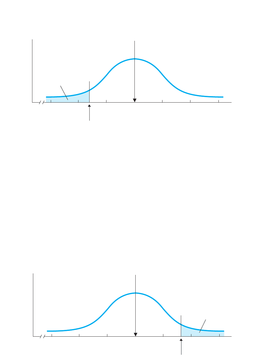
Previously, the region of rejection was in both tails of the distribution because we

wanted to identify unrepresentative sample means that were either too far above or too

far below 500. Instead, however, we can place the region of rejection in only one tail of

the distribution. (In the next chapter, you’ll find out why you would want to use this

“one-tailed” test.)

Say that we are interested only in sample means that are less than 500, having

negative z-scores. Our criterion is still .05, but now we place the entire region

of rejection in the lower, left-hand tail of the sampling distribution, as shown in

Figure 9.6. This produces a different critical value. From the z-table (and using the

interpolation procedures described in Appendix A.2), the extreme lower 5% of a dis-

tribution lies beyond a z-score of Therefore, the z-score for our sample must

lie beyond the critical value of for it to be in the region of rejection. If it

does, we will again conclude that the sample is so unlikely to be representing the

SAT population where that we’ll reject that the sample represents this pop-

ulation. However, if the z-score is anywhere else on the sampling distribution, even

far into the upper tail, we will not reject that the sample represents the SAT popula-

tion where ␮ 5 500.

␮ 5 500

21.645

21.645.

␮

;

21.301474 2 5002>20 521.30.

␮

Deciding Whether a Sample Represents a Population 201

Critical value = –1.645

440

–3

460

–2

480

–1

500

520

540

560

Region of rejection

equals 5%

Sample means

z-scores

FIGURE 9.6

Setup of SAT sampling distribution to test negative z-scores

Critical value = +1.645

440

–3

460

–2

480

–1

500

520

540

560

Region of rejection

equals 5%

Sample means

z-scores

FIGURE 9.7

Setup of SAT sampling distribution to test positive z-scores

On the other hand, say that we’re interested only in sample means greater than 500,

having positive z-scores. Here, we place the entire region of rejection in the upper,

right-hand tail of the sampling distribution, as shown in Figure 9.7. Now the critical

value is plus , so only if our sample’s z-score is beyond does the sample

mean lie in the region of rejection. Only then do we reject the idea that the sample rep-

resents the underlying raw score population.

REMEMBER When using one tail of the distribution and a criterion of

.05, we use only the critical value of or only the critical value

of 21.645.

11.645

11.6451.645

PUTTING IT

ALL TOGETHER

202 CHAPTER 9 / Using Probability to Make Decisions about Data

The decision-making process discussed in this chapter is the essence of all inferential

statistics. The basic question is always “Do the sample data represent a specified raw

score population?” The sample may not look like it represents the population, but that

may simply be sampling error or the sample may represent some other population. To

decide, we

1. Draw a sampling distribution for the specified underlying raw score population.

2. Select the criterion probability, determine the critical value, and label your

distribution, showing the region of rejection.

3. Compute a z-score for the sample mean.

4. If is beyond the critical value, it is in the region of rejection. Therefore, the

sample is unlikely to represent the underlying raw score population, so reject that

it does. Conclude that the sample represents another population that is more likely

to produce such data.

5. If is not beyond the critical value, then the sample is not in the region of

rejection and is likely to merely reflect sampling error. Therefore, retain the idea

that the sample represents the specified population, although somewhat poorly.

With these steps, we make an intelligent bet about the population that our sample rep-

resents. Recognize that, as with any bet, our decisions might be wrong. (We’ll discuss

this in the next chapter.) Such errors are not likely, however, and that is why we per-

form inferential procedures. By incorporating probability into our decision making, we

■

To decide if a sample represents a particular raw

score population, compute the sample mean’s

z-score and compare it to the critical value on the

sampling distribution.

MORE EXAMPLES

A sample of SAT scores produces

Does the sample represent the SAT population where

and ? Compute

;

With a criterion of .05 and the region of rejec-

tion in both tails, the critical value is The

sampling distribution is like Figure 9.5. The of

is beyond , so it is in the region of rejection.

Conclusion: The sample does not represent this SAT

population.

For Practice

1. The region of rejection contains those samples

considered to be likely/unlikely to represent the

underlying raw score population.

21.96

22z

;1.96.

22.0.

z 5 1X

2 ␮2>σ

5 1460 2 5002>20 5100>125 5 20

z: σ

5 σ

>1N 5σ

5 100␮ 5 500

X 5 460.1N 5 252

2. The ____ defines the z-score that is required for a

sample to be in the region of rejection.

3. For a sample to be in the region of rejection, its

z-score must be smaller/larger than the critical

value.

4. On a test, and A sample

produces Using the .05

criterion and both tails, does this sample

represent this population?

Answers

1. unlikely

2. critical value

3. larger (beyond)

4. ;

this is beyond , so reject that the sample

represents this population; it’s likely to represent the

population with ␮ 5 65.

;1.96z

z 5 165 2 602>1.80 512.78.σ

5 18>2100 5 1.80

X 5 65.1N 5 1002

5 18.␮ 5 60

A QUICK REVIEW

Key Terms 203

CHAPTER SUMMARY

1. Probability indicates the likelihood of an event when random chance is operating.

2. Random sampling is selecting a sample so that all elements or individuals in the

population have an equal chance of being selected.

3. The probability of an event is equal to its relative frequency in the population.

4. Two events are independent if the probability of one event is not influenced by the

occurrence of the other. Two events are dependent if the probability of one event

is influenced by the occurrence of the other.

5. Sampling with replacement is replacing individuals or events back into the

population before selecting again. Sampling without replacement is not replacing

individuals or events back into the population before selecting again.

6. The standard normal curve is a theoretical probability distribution. The proportion

of the area under the curve for particular z-scores is also the probability of the

corresponding raw scores or sample means.

7. In a representative sample, the individuals and scores in the sample accurately

reflect the types of individuals and scores found in the population.

8. Sampling error results when chance produces a sample statistic (such as ) that is

different from the population parameter (such as ) that it represents.

9. The region of rejection is in the extreme tail or tails of a sampling distribution.

Sample means here are unlikely to represent the underlying raw score population.

10. The criterion probability is the probability (usually .05) that defines samples as

unlikely to represent the underlying raw score population.

11. The critical value is the minimum z-score needed for a sample mean to lie in the

region of rejection.

␮

1p2

KEY TERMS

criterion probability 198

critical value 198

dependent event 189

independent event 188

inferential statistics 186

probability 187

probability distribution 188

random sampling 186

region of rejection 197

representative sample 193

sampling error 193

sampling with replacement 189

sampling without replacement 189

are confident that over the long run we will correctly identify the population that a

sample represents. In the context of research, therefore, we have greater confidence that

we are interpreting our data correctly.

204 CHAPTER 9 / Using Probability to Make Decisions about Data

REVIEW QUESTIONS

(Answers for odd-numbered questions are in Appendix D.)

1. (a) What does probability convey about an event’s occurence in a sample?

(b) What is the probability of a random event based on?

2. What is random sampling?

3. (a) What is sampling with replacement? (b) What is sampling without

replacement? (c) How does sampling without replacement affect the probability of

events, compared to sampling with replacement?

4. (a) When are events independent? (b) When are they dependent?

5. What does the term sampling error indicate?

6. When testing the representativeness of a sample mean, (a) What is the criterion

probability? (b) What is the region of rejection? (c) What is the critical value?

7. What does comparing a sample’s z-score to the critical value indicate?

8. What is the difference between using both tails versus one tail of the sampling

distribution in terms of (a) the size of the region of rejection? (b) the critical

value?

APPLICATION QUESTIONS

9. Poindexter’s uncle is building a house on land that has been devastated by

hurricanes 160 times in the past 200 years. However, there hasn’t been a major

storm there in 13 years, so his uncle says this is a safe investment. His nephew

argues that he is wrong because a hurricane must be due soon. What are the

fallacies in the reasoning of both men?

10. Four airplanes from different airlines have crashed in the past two weeks. This

terrifies Bubbles, who must travel on a plane. Her travel agent claims that the

probability of a plane crash is minuscule. Who is correctly interpreting the

situation? Why?

11. Foofy conducts a survey to learn who will be elected class president and

concludes that Poindexter will win. It turns out that Dorcas wins. What is the

statistical explanation for Foofy’s erroneous prediction?

12. (a) Why does random sampling produce representative samples? (b) Why does

random sampling produce unrepresentative samples?

13. In the population of typical college students, on a statistics final exam

For 25 students who studied statistics using a new technique,

Using two tails of the sampling distribution and the .05 criterion:

(a) What is the critical value? (b) Is this sample in the region of rejection?

How do you know? (c) Should we conclude that the sample represents the

population of typical students? (d) Why?

14. In a population, and A sample has Using

two tails of the sampling distribution and the .05 criterion: (a) What is the critical

value? (b) Is this sample in the region of rejection? How do you know? (c) What

does this indicate about the likelihood of this sample occurring in this population?

(d) What should we conclude about the sample?

15. The mean of a population of raw scores is Use the criterion of

.05 and the upper tail of the sampling distribution to test whether a sample with

represents this population. (a) What is the critical value?

(b) Is the sample in the region of rejection? How do you know? (c) What does this

X 5 36.8 1N 5 302

33 1σ

5 122.

X 5 102.1N 5 1502σ

5 25.␮ 5 100

X 5 72.1.

1σ

5 6.42.

␮ 5 75

Integration Questions 205

indicate about the likelihood of this sample occurring in this population? (d) What

should we conclude about the sample?

16. We obtain a which may represent the population where

Using the criterion of .05 and the lower tail of the sampling dis-

tribution: (a) What is our critical value? (b) Is this sample in the region of rejection?

How do you know? (c) What should we conclude about the sample? (d) Why?

17. The mean of a population of raw scores is Your is 34 (with

Using the .05 criterion with the region of rejection in both tails of the

sampling distribution, should you consider the sample to be representative of this

population? Why?

18. The mean of a population of raw scores is Your is 44 (with

Using the .05 criterion with the region of rejection in both tails of the

distribution, should you consider the sample to be representative of this

population? Why?

19. A couple with eight daughters decides to have one more baby, because they think

this time they are sure to have boy! Is this reasoning accurate?

20. On a standard test of motor coordination, a sports psychologist found that the

population of average bowlers had a mean score of 24, with a standard deviation

of 6. She tested a random sample of 30 bowlers at Fred’s Bowling Alley and

found a sample mean of 26. A second random sample of 30 bowlers at Ethel’s

Bowling Alley had a mean of 18. Using the criterion of and both tails of

the sampling distribution, what should she conclude about each sample’s

representativeness of the population of average bowlers?

21. (a) In question 20, if a particular sample does not represent the population of

average bowlers, what is your best estimate of the of the population it does

represent? (b) Explain the logic behind this conclusion.

22. Foofy computes the from data that her professor says is a random sample from

population Q. She correctly computes that this mean has a z-score of on the

sampling distribution for population Q. Foofy claims she has proven that this could

not be a random sample from population Q. Do you agree or disagree? why?

INTEGRATION QUESTIONS

23. In a study you obtain the following data representing the aggressive tendencies of

some football players:

40 30 39 40 41 39 31 28 33

(a) Researchers have found that in the population of nonfootball players, is 30

Using both tails of the sampling distribution, determine whether your

football players represent a different population. (b) What do you conclude about

the population of football players and its ? (Chs. 4, 6, 9)

24. We reject that a sample, with , is merely poorly representing the population

where (a) What is our best estimate of the population that the sample

is representing? (b) Why can we claim this value of ? (Ch. 4)

25. For a distribution in which and , using z-scores, what is the relative

frequency of (a) scores below 27? (b) Scores above 51? (c) A score between 42

and 44? (d) A score below 33 or above 49? (e) For each of the questions above,

what is the probability of randomly selecting participants who have these scores?

(Chs. 6, 9)

5 8X 5 43

␮

␮␮ 5 100.

X 5 95

␮

1σ

5 5.2

␮

141

␮

p 5 .05

N 5 402.

X48 1σ

5 162.

N 5 352.

X28 1σ

5 92.

␮ 5 50 1σ

5 112.

X 5 46.8 1N 5 152

206 CHAPTER 9 / Using Probability to Make Decisions about Data

26. When we compute the z-score of a sample mean, (a) What must you compute

first? (b) What is its formula? (c) What is the formula for the z-score of a sample

mean? (d) It describes the mean’s location among other means on what

distribution? (e) What does this distribution show? (Chs. 6, 9)

27. The mean of a population of raw scores is (a) Using the z-table,

what is the relative frequency of sample means below 46 when ?

(b) What is the probability of randomly selecting a sample of 40 scores

having a below 46? (Chs. 6, 9)

28. The mean of a population of raw scores is (a) Using the z-table,

what is the relative frequency of sample means above 24 when ? (b) What

is the probability of randomly selecting a sample of 30 participants whose scores

produce a mean above 24? (Chs. 6, 9)

N 5 30

18 1σ

5 122.

N 5 40

50 1σ

5 182.

■ ■ ■ SUMMARY OF

FORMULAS

1. The formula for transforming a sample mean into

a z-score is

z 5

2 ␮

where the standard error of the mean is

207

Introduction to

Hypothesis Testing

GETTING STARTED

To understand this chapter, recall the following:

■

From Chapter 2, what the conditions of an independent variable are and what

the dependent variable is.

■

From Chapter 4, that a relationship in the population occurs when different

means from the conditions represent different and thus different distributions

of dependent scores.

■

From Chapter 9, that when a sample’s z-score falls into the region of rejection,

the sample is unlikely to represent the underlying raw score population.

Your goals in this chapter are to learn

■

Why the possibility of sampling error causes researchers to perform inferential

statistical procedures.

■

When experimental hypotheses lead to either a one-tailed or a two-tailed test.

■

How to create the null and alternative hypotheses.

■

How to perform the z-test.

■

How to interpret significant and nonsignificant results.

■

What Type I errors, Type II errors, and power are.

␮s

From the previous chapter, you know the basic logic of all inferential statistics.

Now we will put these procedures into a research context and present the statistical

language and symbols used to describe them. Until further notice, we’ll be talking

about experiments. This chapter shows (1) how to set up an inferential procedure,

(2) how to perform the z-test, (3) how to interpret the results of an inferential proce-

dure, and (4) the way to describe potential errors in our conclusions.

NEW STATISTICAL NOTATION

Five new symbols will be used in stating mathematical relationships.

1. The symbol for greater than is . Thus, means that is greater than .

2. The symbol for less than is , so means that is less than .

3. The symbol for greater than or equal to is , so indicates that is greater

than or equal to .

4. The symbol for less than or equal to is , so indicates that is less than

or equal to .

5. The symbol for not equal to is so means that is different from .BAA ? B?,

BB # A#

BB $ A$

ABB 6 A6

BAA 7 B7