Heard D.E. (editor) Analytical Techniques for Atmospheric Measurement

Подождите немного. Документ загружается.

32 Analytical Techniques for Atmospheric Measurement

College of Marine Studies (http://www.researchvessels.org/). Ship-borne platforms have

the advantage that heavy and power-hungry instruments can be accommodated, although

space in laboratories is limited. Some ships have deck space for shipping containers,

enabling larger instruments to be deployed. Cruises may last for long periods, several

months at a time, and thus very long time-series can be measured, providing latitudinal

gradients of key species from polar to equatorial regions. Care must be taken that the

sampling is forward of the exhaust stack, and that local wind-fields are well understood.

Pseudo-Langragian experiments have been performed in which an instrumented ship

is positioned either upwind or downwind of a ground-based site, with connected flow

between the sites allowing the chemical evolution of a given airmass to be followed

from measurements in changes in composition. Alternatively, measurements along a

ship-track away from an ocean upwelling hotspot will enable the atmospheric processing

of marine emissions to be studied. It is possible for ice-breakers to remain locked in

the ice during polar winters, and to obtain seasonal changes in composition during the

transition from winter to spring to summer as the sea-ice cracks, breaks up and disperses.

Ship measurements are also useful for satellite validation.

1.4.3 Balloon-borne platforms

In situ instruments deployed on the platforms considered in Sections 1.4.1 and 1.4.2 do

not allow for vertically resolved measurements, and although remote sensing techniques

can provide some information of this type, it is often limited by scattering and absorption

of light in the boundary layer. Balloons represent a relatively simple and inexpensive

solution to this problem. Small (weather) balloons carrying a lightweight radiosonde

(up to a few kg) have been used in their thousands to obtain profiles of meteorological

parameters (pressure, temperature, humidity, wind direction and speed). An ozonesonde

is also commonly deployed on balloons as part of an international network, and consists

of an I

−

(aq) electrochemical cell (see Section 1.5.3) to measure ozone, and aerosols

have also been measured using small instruments. Many stations worldwide release a fixed

number of balloons each day to obtain a long-term record. The balloons are constant-

pressure devices (the pressure inside the balloon is the same as ambient pressure),

containing a fixed mass of helium, with thin membranes that expand as the balloon

ascends, according to the ideal gas equation:

pV = nRT (1.5)

where p and T are ambient pressure and temperature, n is the (fixed) number of moles

of helium (1 mole contains 602 ×10

molecules) and V is the balloon volume. Data

are sent back to the ground via telemetry, with the balloons eventually bursting and the

sonde (usually not recovered) falling back to earth.

To lift heavier instruments, a larger balloon is required, as more lift can be generated

by a larger volume of the lighter helium. Scientific balloons can be very large (up to

) and are able to lift payloads of up to ∼ 1000kg to altitudes of 30–45 km. There

are severe constraints on the instruments – they must be automatic and capable of

withstanding wide ranges of pressures and temperatures. Instrument packages are often

Field Measurements of Atmospheric Composition 33

contained with gondolas that may be up to 100 m or more below the balloon, so that the

instruments are not shaded by the balloon. Weather conditions have to be perfect for

launch, and this limits the deployment of balloon instruments. Long duration balloons

that fly for several weeks are able to circumnavigate the globe one or more times, and

drift with the wind at an almost constant altitude. Such balloons have been used in the

tropics to measure trace species involved in stratospheric ozone depletion that have been

transported from the surface to the tropopause by deep convection, and are ideal for

satellite validation. The history of constant-level balloons as observational platforms for

atmospheric research has been reviewed by Businger et al. (1996). Much reliance is placed

on global positioning systems to record the precise flight track, and instruments include

lightweight instruments to measure O

and H

O vapour.

Tethered balloons are also quite widely used, with payloads of a few kg, although their

altitude ceiling is limited to about 1500 m because of the weight of the tethering cable, but

with a winching device the height of the instrument payload can be precisely changed.

1.4.4 Aircraft-borne platforms

Aircraft are an excellent means to obtain a three-dimensional distribution of trace gases

and aerosols in the atmosphere, on account of their high speed, long range and ability to

sample a range of altitudes quickly. Space is usually at a premium and hence instruments

must be lightweight and compact, must not generate radio-frequency emissions that

may interfere with aircraft avionics, and ideally should use small amounts of electrical

power, although larger aircraft can generate significant power (but initially at a rather

inconvenient frequency of 400 Hz, and this has to be converted to 50 Hz 240 V a.c.

or 28 V d.c.). There are greater demands on instruments on aircraft, which should

be designed to withstand high stress loadings. Research aircraft vary from the small,

for example a Cessna single-engined turboprop aircraft, with a relatively low ceiling

(13 500 feet), low range (∼1000 km) and short duration (∼6 h), all the way to large

civil airliners, for example the highly-modified four jet-engined McDonnell Douglas

DC-8 that is operated by NASA. The NASA DC-8 has a very large instrument payload

(13 600 kg), has a flight duration of 12 h, can fly from 1000 to 42 000 feet (13.7 km),

and has a range of 10 000 km. It is beyond the scope of this introductory chapter to

list in detail the performance specification of all the research aircraft in use today, but

further sources of information can easily be found on the Internet. Some of the larger

fully instrumented aircraft, in addition to the NASA DC-8, are the NASA WB-57 (18 km

ceiling), the UK BAe-146 (Facility for Airborne Atmospheric Measurements, FAAM), the

M-55 Geophysica (initially Russian Air Force, 21 km ceiling), the NASA Lockheed ER-2

aircraft (converted U-2 series reconnaissance platform, 21 km ceiling, 1200 kg payload),

the Lockheed P3-B (operated by several agencies), the Lockheed Hercules C-130 series

transport aircraft (12 hr endurance, 17 000 kg scientific payload, capable of flying at 50 feet

over water), the German DLR Falcon 20 and French Mystere Falcon 20.

There have been many aircraft-based field campaigns, and some of these are listed in

Table 1.3. Co-ordination with other research aircraft is a feature of field campaigns, and

it has been possible to follow the chemical evolution and photochemical processing of

identified plumes over very large distances. An example is the ICARTT (International

Consortium for Atmospheric Research on Transport and Transformation) project, which

34 Analytical Techniques for Atmospheric Measurement

monitored the export of polluted layers from North America across the North Atlantic

towards Europe. Four NASA and NOAA research aircraft were based on the US eastern

seaboard (as was the Ronald H. Brown research vessel), the UK BAe-146 was based on

the mid-Atlantic island of Faial in the Azores, and the German Falcon aircraft was based

at Creil, France.

Essential to the flight planning and scientific design of aircraft sorties are forecast

modelling tools; for example, reverse domain filling trajectories, which predict at any time

for a given flight path the origin of the sampled air. Inlet systems should ideally be close

to the front of the aircraft, as the skin boundary layer increases in width along the length

of the fuselage. Satellite validation is becoming a more important part of aircraft field

campaigns as the range of species monitored by satellites in the troposphere increases

(see Section 1.4.8).

1.4.5 Commercial passenger or freight aircraft platforms

Analysing atmospheric trace gases and aerosols using commercial passenger aircraft repre-

sents a cost-effective solution for recording many thousands of hours of flight data. The

main advantage being that near-global coverage is possible, as opposed to limited coverage

using a limited number of research aircraft. Other applications include comparison with

satellite measurements along the flight-paths or land-based observatories close to take-off

and landing. There are currently three passenger aircraft systems operating worldwide,

which have been reviewed in 2005 (Brenninkmeijer et al., 2005), and from which much

of the material in this section has been taken. The certification of equipment for use

on passenger aircraft by aviation authorities can be a lengthy process. Most of the data

are taken at cruising altitudes of 9–12 km, and for mid-latitudes, stratospheric air is

sometimes sampled.

The EU-funded Civil Aircraft for the Regular Investigation of the Atmosphere Based

on an Instrument Container (CARIBIC, www.caribic-atmospheric.com) project began

in 1997; it used an automated container deployed on intercontinental flights using a

Boeing 767, but now a more powerful instrument package is deployed using a new Airbus

A340-600 operated by Lufthansa. There are 1–2 flights per month, and measurements

(technique and chapter number in brackets) include the following:

•

(chemiluminescence, 7, and UV absorption, 3)

•

CO (Vacuum UV fluorescence, 4; gas chromatography and a reducing gas detector, 8)

O vapour (diode laser photoacoustic detection, 2)

•

NO and NO

(chemiluminescence, 7) mercury vapour (atomic fluorescence, 4)

•

(non-dispersed IR absorption, 2)

•

(electrochemical cells, 1)

•

methanol, acetone, acetaldehyde (proton transfer mass spectrometry, 5)

•

aerosols (>4nm>12nm>18nm, condensation particle counter, 6)

•

aerosol size distribution (15–5000 nm, optical particle counter, 6)

•

aerosol elemental composition (filter impactor, 6)

•

particle morphology (impactor, electron microscopy, 8)

Field Measurements of Atmospheric Composition 35

•

non-methane hydrocarbons, halocarbons, CO

,CH

O, SF

(whole air sampler with

28 glass flasks, analysis by GC and GC-MS, 5 and 8)

•

oxygenated VOCs (adsorption tubes followed by GC analysis, 8)

•

BrO, HCHO, OClO, O

dimer, all remote sensing DOAS, 3)

•

cirrus clouds.

Measurement of

OZone and water vapour by Airbus In-service Aircraft (MOZAIC,

www.aero.obs-mip.fr/mozaic) is an EU-funded network of five Airbus 340–300 aircraft

that contain in situ instruments for the measurement of O

O vapour, NO

(= NO

+HNO

+HONO +alkyl nitrates +PAN) and CO. Measurements of aerosols

are planned. Between September 1994 and June 2004 there have been 20 960 flights and

160 000 flight hours made over the continents of Europe, North America, Asia, South

America, Africa and the Atlantic Ocean, and hence there is a fantastic dataset for use by

the atmospheric community.

The JAL Foundation (www.jal-foundation.or.jp/) has funded the collection of air flask

samples from a Japan Airlines Boeing 747, mainly on routes between Japan and Australia,

and expansion is underway to involve seven 747-400 and 777 aircraft (flask sampling and

in situ CO

measurements).

1.4.6 Uninhabited aerial vehicles

Uninhabited aerial vehicles (UAVs) have undergone considerable development, driven

primarily for military use. They offer considerable advantages where manned craft are

dangerous or difficult to deploy, or for very long missions when pilot fatigue is a limiting

factor. UAVs have also been used for a variety of atmospheric monitoring applications.

In situ measurements of vertical profiles of the composition of the atmosphere in regions

where current aircraft cannot reach are needed to validate and calibrate satellite measure-

ments. The US National Oceanic and Atmospheric Administration (NOAA) have tested

(May 2005) an Altair UAV, which is a high altitude version of the Predator UAV, whose

payload includes a gas chromatograph for measurements every 70 seconds of long-

lived gases – SF

, nitrous oxide (N

O), CFC-11 (CFCl

), CFC-12 (CF

) and H-1211

(CBrClF

) – and a UV absorption instrument for measurement of O

. The vertical distri-

bution of water vapour has been remotely measured with passive microwave sensors. The

altitude ceiling of this UAV is ∼15 km; it has a combined internal and external payload

of ∼1500 kg, and a duration of 30 hours. Further information on this demonstration

project can be found at http://uav.noaa.gov/index.html.

1.4.7 Rocket platforms

The maximum altitude for balloons is about 45 km, and in situ measurements for vertical

profiles at higher altitudes have been achieved with rockets, which have payloads of

up to few 100 kg and can reach 200–300 km. The rockets are recovered after use, and

hence must be launched from remote locations; for example, from Andoya, on the

Norwegian Coast (rockets reovered from the ocean), Wallops Island, Virginia, USA and

36 Analytical Techniques for Atmospheric Measurement

White Sands, New Mexico, USA. Rocket-based measurements of the hydroxyl radical

have been made between 45 and 70 km altitude in the mesosphere using solar-induced

fluorescence spectroscopy, with ∼ 2km vertical resolution. Measurements can be during

the rocket ascent (lasting only a few minutes) or during a slower descent below a

parachute.

1.4.8 Satellites and other space-borne platforms

The use of satellites represents one of the most important advances in the monitoring

of our atmosphere. Measurements of atmospheric composition from space have revolu-

tionised our understanding of the three-dimensional distribution of trace gases in the

atmosphere and of the impact humans have had on it. Satellites have enabled direct obser-

vation of intercontinental long-range transport of biogenic and anthropogenic emissions

and the global observation of regulatory species over periods of several years. An example

is ozone, whose tropospheric background levels have steadily risen as a result of the

oxidative processing of VOCs in the presence of NO

during long-range transport.

Sources of emission (urban areas) may be thousands of kilometres away from the regions

of resulting elevated ozone. Satellite data have shown unequivocally that pollution is a

global issue, and provide a direct comparison with the output from CTMs, enabling

their realistic evaluation. Satellite data will allow the following questions to be answered:

Will the recovery of the ozone layer follow the model predictions, or will it be altered

because of cooling in the stratosphere caused by greenhouse gases? What is controlling the

concentrations of tropospheric pollutants? What is the impact of changes in atmospheric

composition, for example upper tropospheric aerosols, ozone and water vapour, on

climate?

This book is organised according to analytical technique, each of which has been

deployed on a number of platforms, and hence there is no chapter dedicated to the use

of satellite platforms. In this section, no attempt is made to provide a comprehensive

treatment of satellite instruments and methods, rather a summary is given of the satellite

platforms available, their orbits and viewing geometries, the temporal coverage and

vertical resolution, a description of some of the instruments and the species that have

been measured. The subject of satellite measurements is now very large indeed, with

numerous satellites in orbit equipped with arrays of instruments, and the volume of data

becoming available is truly enormous. Further information can be found in Brasseur

et al. (1999, 2003), Burrows (1999), Calvert (1994), Platt & Stutz (2006), Scott (2005),

and from a number of excellent Web pages, for example:

http://jwocky.gsfc.nasa.gov/ (TOMS)

http://www-iup.physik.uni-bremen.de/gome/ (GOME)

http://www-iup.physik.uni-bremen.de/sciamachy/index.html (SCIAMACHY)

http://envisat.esa.int/instruments/tour-index/mipas/ (MIPAS)

http://www.eos.ucar.edu/mopitt/ (MOPITT)

http://www-sage2.larc.nasa.gov/ (SAGE II)

http://eos-aura.gsfc.nasa.gov/ (AURA)

Field Measurements of Atmospheric Composition 37

Additional references are given below and further information on satellites and their data

products can be obtained from the Internet.

Satellite instruments rely on passive remote sensing of scattered or transmitted sunlight,

or emitted thermal or microwave radiation (essentially DOAS from space). Chapters 2

and 3 describe the techniques of IR absorption spectroscopy and UV-visible DOAS,

respectively. An excellent resource for the use of DOAS from satellites can be found in

Platt & Stutz (2006). Naturally, there are extreme constraints on satellite instruments, for

example in power consumption, weight, size, reliability, autonomy, resistance to cosmic

radiation. The development costs are very high and there may be many years from

instrument concept to measurement.

Several modes of observation are possible from satellites, which depend both on the

orbit of the satellite and on the viewing angle of the instrument. There are two types

of orbit, geostationary orbit (GEO) and low-earth orbit (LEO). At present, instruments

that use DOAS are all aboard satellites in LEO. The satellite in GEO is 35 790 km from

the earth’s surface, and maintains a constant position with respect to the rotating earth.

Hence the orbital period (time for one orbit) is exactly equal to the period of rotation

of the earth (23 hr, 56 min, 4.09 s). By orbiting at the same rate, in the same direction

as earth, the satellite appears stationary (synchronous with respect to the rotation of

the earth). GEO satellites give the ‘big picture’ view, enabling coverage, for example, of

weather events, and is especially useful for monitoring severe local storms and tropical

cyclones. Being positioned in the equatorial plane, distorted images are provided of polar

regions with poor spatial resolution.

Low-earth orbit satellites enable observation of the entire surface of the earth, but only

for a short period each day. Many satellites are launched into an almost polar orbit,

passing over the North and South Poles, at an altitude of 700–800 km. The satellite

must travel quickly ∼27000 km hr

−1

 relative to the earth so that the centrifugal force

balances the significant gravitational force. The orbit period is 90–100 min, and provides

a thorough coverage of the earth’s surface, which spins ∼ 24



of longitude about its axis

between successive orbits (the observation is akin to peeling an orange in one piece). In a

sun-synchronous orbit, the satellite passes over a given longitude at intervals of 12 hours

(once in the dark), and enables regular data collection at consistent times and long-term

comparisons. The majority of satellites used for compositional measurements use this

type of orbit so that variation with location can be distinguished from variation with time

of day. Inclined orbits have an inclination somewhere between equatorial 0



 and polar

90



 orbit, with a period of a few hours, and are not sun synchronous, passing over a

given location at different times. An example is the Upper Atmosphere Research Satellite

(UARS) which contains six instruments for studies of the chemistry of the stratosphere,

mesosphere and lower thermosphere. Care has to be taken when positioning a satellite.

NASA is tracking more than 8000 objects larger than a cricket ball, all orbiting the earth

at 27 000 km hr

−1

Limb-viewing along a horizontal path or nadir-viewing looking directly below the

satellite are both used and provide complementary information. Limb observations of

sunlight scattered at the horizon provide excellent vertical resolution but poor horizontal

resolution (400 km). Cloud, aerosol and spectral interference make measurements below

8 km very difficult using limb-viewing. Nadir observations of sunlight reflected by earth’s

surface or atmosphere (earthshine) provide better horizontal resolution and are capable

38 Analytical Techniques for Atmospheric Measurement

of detecting down to the earth’s surface. However, the vertical resolution is poor (often

only a column measurement is possible). Other types of observation are solar, lunar and

stellar occultation, where the light source is viewed directly, and absorption through the

atmosphere is measured. In addition thermal emission from excited molecules in the

atmosphere is observed rather than scattered sunlight. The main disadvantages of satellite

measurements are the poor time resolution for a given location (once per day) and the

bias of the measurements towards clear sky conditions.

Some of the species observed from satellites are listed in Table 1.2. A very compre-

hensive listing of species, together with the satellite platform and instrument used, the

the type of orbit, and the altitude range of the measurement, can be found in Platt &

Stutz (2006). Examples of instruments (satellite in brackets) include the Global Ozone

Monitoring Experiment – 2, GOME-2 (ESA ERS-2), Stratospheric Aerosol and Gas

Experiment II, SAGE II (Earth Radiation Budget Satellite), Solar Backscatter Ultraviolet

Ozone Experiment, SBUV (Nimbus-7), Scanning Imaging Absorption Spectrometer for

Atmospheric Cartography, SCIAMACHY (ESA-Envisat), and Total Ozone Monitoring

Spectrometer, TOMS (Earth Probe). The GOME instrument (Burrows et al., 1999) makes

trace gas measurements using four medium resolution spectrometers, in the range of

290–790 nm, each with 1024 channels. The reflected sunlight from the atmosphere is

analysed in nadir mode using the DOAS technique (Chapter 3), and column densities of

, BrO, OClO, SO

O, O

and O

(the weakly bound O

van der Waals dimer) are

reported every 1.5 s. A scanning mirror moving perpendicular to the direction of travel of

the satellite directs light into the spectrometer, and for each spectrum the ‘ground pixel’

(or footprint on the ground) is 320 km ×40 km. The swathe is 960 km wide (3 pixels).

Measurements of stratospheric composition began with O

back in 1970 (with the SBUV

instrument on the Nimbus 4 satellite) and NO

starting in 1979 (Platt & Stutz, 2006).

One of the workhorses over the years has been the TOMS instrument, which measures

the total column of O

, and which first demonstrated clearly the extent of the ozone

hole over Antarctica. The instrument (Heath et al., 1975) consists of a grating UV-visible

spectrometer, and six wavelengths are monitored between 213 and 380 nm, where few

other molecules absorb. A disadvantage is that no measurements are possible for the

polar night, but the instrument can also measure SO

(strong absorption features in the

same spectral region), and has tracked plumes emanating from volcanoes and reaching

the stratosphere. Another example is stratospheric OClO, which is a good indicator of

chlorine activation.

Measurements of trace gases and aerosols in the troposphere from satellites are a more

recent phenomenon, and are much more difficult than those in the upper atmosphere.

The presence of clouds means that virtually all measurements are made using the nadir-

viewing geometry, with poor vertical resolution. Obtaining the tropospheric contribution

to the total column is especially difficult for species that are highly abundant in the

stratosphere, for example O

(only ∼10% of the total column is from the troposphere)

and NO

. For other species, for example HCHO, water vapour and SO

, the column

absorption is dominated by tropospheric contributions. There are several procedures

(retrieval methods) for separating out the ‘stratospheric’ signal for species abundant

in the stratosphere. The multi-step reference sector method (used for NO

) compares

signals from regions where it is known that there are no tropospheric contributions to

the total NO

column with signals from polluted regions, with the difference giving the

Field Measurements of Atmospheric Composition 39

tropospheric NO

column. In the cloud slicing method the difference between columns

measured above clouds and in cloud-free conditions is used to get the tropospheric

contribution. The spectral line shape of an absorption feature is a function of temperature

and pressure, and hence its careful observation can be used to extract a vertical profile.

Finally, the difference in column amounts between two satellite instruments viewing the

same point, but with one sensitive only to stratospheric altitudes, has been used to obtain

troposphere columns, for example for O

(Fishman et al., 1990). The retrieval algorithms

are extremely complex and time-consuming, and must be developed for each separate

species of interest. The absorption pathlength in the troposphere will depend upon the

height above sea level, and for high-precision measurements of long-lived species which

are well mixed (e.g. CO

and CH

) and which have fairly uniform concentrations, the

presence of mountain ranges must be taken into account.

Some of the first measurements of tropospheric CO, produced as a result of incomplete

combustion during burning processes, and a good indicator of atmospheric pollution,

were made by the Measurement of Air Pollution from Satellites (MAPS) instrument in

1984 from the space shuttle, whereas tropospheric O

was first determined in 1977 as a

difference of measurements from SAGE and TOMS instruments. The Measurements of

Pollution in the Troposphere (MOPITT) instrument aboard the Terra satellite has been

used for tropospheric CO and CH

measurements in the near-IR and IR regions. The

MOPITT instrument operates both at short wavelengths, where absorption of reflected

sunlight provides the total CO column, and in the fundamental CO vibrational 1–0

band (48m), where middle and upper tropospheric amounts of CO are determined

(Drummond & Mand, 1996). Subtraction allows determination of concentrations near

the surface. Gas filters containing CO at different pressures (for selective absorption of

radiation from different altitudes) are used to achieve some vertical resolution, so very

high spectral resolution is not required. Retrieval methods in the near-IR and IR have

to take into account the temperature and pressure dependence of the spectral lines, and

there are many overlapping bands from multiple species (in particular water vapour).

Newer instruments such as GOME, SCIAMACHY and TES (Tropospheric Emission

Spectrometer, deployed on the NASA EOS-CHEM Aura satellite) make high quality

tropospheric measurements. The SCIAMACHY instrument makes measurements in limb,

nadir and occultation modes, and uses spectral bands all the way from 240 nm to 2380 mm

to measure tropospheric column amounts of O

,CH

O, SO

, BrO, NO

O, CO,

and N

O (Bovensmann et al., 1999). Vertically resolved concentrations of O

O and CH

will also be measured. The spectrometers aboard GOME only extend to

790 nm, and the ground-footprint of SCIAMACHY for nadir-viewing is also superior

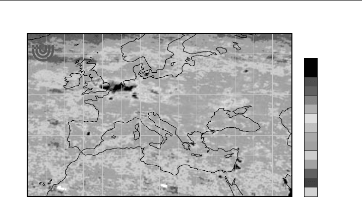
30 km ×60 km. Figure 1.8 shows a map of the tropospheric NO

column for Europe in

August 2002 retrieved from SCIAMACHY DOAS measurements. NO

is emitted directly

and can also be generated through the reactions of HO

and RO

radicals (R is an organic

group, for example CH

) with NO, which is emitted by industrial and transport sources,

and there is a clear correlation between industrial regions and elevated levels of NO

Global maps of tropospheric NO

show peaks over industrialised regions and cities, with

the highest levels globally observed over China. It is also possible to observe ship tracks

from satellites through NO

signatures. Fuel oil used by ships is largely unregulated and

contains high levels of nitrogen and sulphur, resulting in high levels of NO

and SO

being emitted.

40 Analytical Techniques for Atmospheric Measurement

SCIAMACHY tropospheric NO

: 08.2002

VC NO

[molec cm

–2

]

–20 –15 –10 –5 0 5 10 15

Longitude

Latitude

5.0 10

4.0 10

3.0 10

2.0 10

1.0 10

0.0 10

–1.0 10

20 25 30 35 40 45 50

UNIVERSITÄT

BREMEN

Figure 1.8 Tropospheric vertical column for NO

over Europe measured by the SCIAMACHY instrument

aboard the ENVISAT satellite. The pixel size is 30 ×60 km, and the retrieval used the reference sector

method. (Reproduced with permission from Richter et al., 2004, 2005, University of Bremen.) (Reproduced

in colour as Plate 1 after page 264.)

Although at the moment it is not possible to measure global distributions of short-lived

free-radicals (e.g. OH, HO

,RO

,NO

 in the troposphere from space, it is possible to

observe markers of recent photochemical activity. An example is formaldehyde, CH

which is formed from the OH radical-initiated oxidation of methane and other hydro-

carbons, and also during biomass burning. High levels of CH

O have been observed over

forests or regions where there are high levels of biogenic hydrocarbons, such as isoprene

and monoterpenes.

Finally, in polar regions, enhanced levels of BrO, a short-lived halogen species formed

in the oxidation of Br atoms by ozone, have been observed by GOME (Richter et al., 2002;

Wagner & Platt, 1998) and SCIAMACHY. The levels are consistent with concentrations

measured on the ground, and concentrations which occur at the same time as ozone

depletion events (Bottenheim et al., 1990). The BrO levels peak following the long polar

winter in regions containing sea-ice, and disappear once the sea-ice melts. The area of

the BrO clouds is very large, and an autocatalytic mechanism (the so-called ‘bromine

explosion’) has been postulated which involves the oxidation on the sea-ice of Br

−

aq

in sea salt, followed by the release of active bromine compounds.

The NASA space shuttle has also been used to provide measurements from space,

although limited to short durations. The MAPS instrument made measurements of CO in

the 1980s using IR absorption. The Atmospheric Trace Molecular Spectroscopy (ATMOS)

instrument, a high-resolution 0015 cm

−1

 Fourier transform spectrometer, has also flown

on four missions on the Space Shuttle and on Spacelab-3, making measurements in

occultation of solar radiation after it has passed through the atmosphere at sunrise or

sunset (Brasseur et al., 1999). The interferograms are radioed to a receiving station on

the ground where a fast Fourier transformation is performed to yield absorption spectra,

Field Measurements of Atmospheric Composition 41

which are normalised using a spectrum taken above the atmosphere to eliminate structure

from the solar spectrum and instrumental effects. Vertical resolution is possible, and

profiles of almost 40 species have been measured, including in the upper troposphere.

The hydroxyl radical has also been detected using solar-induced fluorescence in the



v



= 0−X



v



= 0 band near 309 nm, and measured as a function of latitude

(50



Sto61



N) and altitude (40–93 km) by the Middle High Resolution Spectrograph

Investigation (MAHRSI) instrument (limb scanning with ∼002nm resolution) on the

Space Shuttle.

Determination of atmospheric composition is not limited to our own atmosphere, and

measurements have been made in the atmospheres of other planets and moons, using

both remote sensing and in situ instruments. An example is the Huygens probe, released

from the Cassini spacecraft, which measured vertically resolved concentrations of trace

gases and aerosols (from 160 km to the surface) in the atmosphere of Titan, a moon of

Saturn, on 25 December, 2004. The composition of aerosols was determined by pyrolysis

and a gas chromatograph with mass spectrometric detection. Initial results confirmed that

the atmosphere is composed mainly of CH

and N

, with CH

concentrations increasing

close to the surface, with clouds of CH

and C

observed, and the presence of

suggests volcanic activity. However, further description of these instruments is beyond

the scope of this book.

1.5 Analytical methods not covered elsewhere

in this book

Inevitably there are analytical methods which do not neatly fall under the headings

used to structure the remainder of this book, but are important to cover nonetheless,

as they provide unique information about the composition of the atmosphere. In this

section, methods not covered elsewhere in this book to make composition measure-

ments in the atmosphere are discussed, but not at the level of detail found in other

chapters. Novel methods only tested in the laboratory are not covered, but brief mention

of promising methods is made in Section 1.10. References are provided for further

information.

1.5.1 LIDAR methods

The power of Light Detection and Ranging (LIDAR) methods is the ability to provide

altitude profile information. Differential Absorption Lidar (DIAL) operates in a similar

manner to DOAS (Chapter 3). Laser light is transmitted at two wavelengths into the

atmosphere, one wavelength tuned to an absorption feature of the species under inter-

rogation, and one wavelength tuned slightly off-resonance with there is little absorption.

Both wavelengths are backscattered by Rayleigh scattering, but the return signal is stronger

for the wavelength that is not absorbed. By using a pulsed laser and the fact that light

travels 300 m in a microsecond, measuring the time delay between the outgoing laser

radiation and the return signal, a vertical profile can be built up of the absorbing species.

LIDAR has been used to measure NO

O vapour, O

, aerosol and SO

(e.g. in stack