Heard D.E. (editor) Analytical Techniques for Atmospheric Measurement
Подождите немного. Документ загружается.


82 Analytical Techniques for Atmospheric Measurement
Figure 2.5 A low-resolution display of vibrational-rotational lines of four major atmospheric constituents
in the 2000 to 3200 cm
−1
window under the conditions displayed in the plot.
of other species in the lower troposphere. High resolution spectra for the specific regions
of interest, however, are further required to determine if these abundant gases will present
a problem.
Table 2.1 and the references cited above illustrate the sheer number of atmospheric
constituents that absorb in the mid-IR spectral region. This is in contrast to the visible and
UV spectral regions, where significantly fewer atmospheric constituents exhibit strong
absorptions. This is one aspect that makes mid-IR absorption measurements a partic-
ularly attractive tool for atmospheric research. However, this is not without unique
measurement challenges. Since many mid-IR atmospheric studies employ laser sources
of one kind or another, advances in mid-IR measurement performance are closely tied to
advances in laser source development. Although there has been a great deal of activity in
this area, progress in mid-IR laser source development has not kept pace with progress in
other regions of the electromagnetic spectrum in terms of performance and ease of use.
In fact, as of this writing, the optimum laser sources reside in the near-IR spectral region,
more particularly in the 09–18 m spectral region, where advances from the telecom-
munications industry have helped push the development. Unfortunately, the number of
atmospheric gases that can be studied in this spectral region are somewhat limited due

Infrared Absorption Spectroscopy 83
Table 2.1 Band origins (rounded to nearest cm
−1
) and integrated band strengths for some of the important
trace gases from Smith et al. (1985) unless otherwise noted. Use strengths as a guide, since in many cases
multiple values are presented by Smith et al. (1985). The bands are for the major isotopes
Molecule Band Band origin cm
−1
S
v
cm
−2
atm
−1
at 300 K
CO 1-0 2143 235
HBr 1-0 2559 55
a
HCl
35
1-0 2886 121
b
HF 1-0 3962 408
b
NO 1-0 1876 113
OH 1-0 3570
CO
2
2
1
667 200
3
2349 2230
HCN
1
2097 0.1
2
712 234
3
3312 219
H
2
O
1
3657 10
a
2
1595 254
3
3756 192
a
N
2
O
1
1285 277
2
1
589 29
3
2224 1173
NO
2
1
1320 2
2
750 13
3
1617 1400
1
+
3
2906 70
O
3
1
1103 10
a
2
701 18
a
3
1042 361
OCS
1
859 27
2
521 12
3
2062 2184
CH
2
O
1
2782 194
2
1746 301
3
1500 45
4
1167 26
5
2843 356
CH
4
1
2917 0.03
2
1534 2
a
3
3019 276
4
1306 136
a
Band strengths from Pugh and Rao (1976).
b
Band strengths taken from Pine et al. (1985).

84 Analytical Techniques for Atmospheric Measurement
to the significantly weaker line strengths. We will further discuss in Section 2.5.1.2 the
performance, attributes, and drawbacks of various laser sources throughout the IR.
The second main challenge of working in the mid-IR spectral region concerns H
2
O
vapor. Water vapor mixing ratios can be very high and highly variable; typical mixing
ratios can vary from 0.04 (40 000 parts per million by volume, ppmv) to the 10
−6
range
(1 ppmv). Although one has to worry about overtone and combination bands of H
2
O
in the visible and UV spectral regions (electronic transitions occur in the vacuum UV),
absorption line strengths here are typically very weak (in the 10
−26
range with some
lines as strong as 10
−24
). By contrast, discrete strong lines of H
2
O appear throughout
the mid-IR spectral region. Absorption lines in the very strong fundamental bending
vibration shown in Figure 2.4 (band origin 1595 cm
−1
), for example, are as strong as
29 ×10
−19
cm
2
cm
−1
molecule
−1
at 296 K. This coupled with the very high mixing ratios
and the reasonably large air and self-broadening coefficients (to be discussed) adds to
the challenges of quantitative mid-IR absorption measurements. One has to worry about
direct spectroscopic interference not only from H
2
O (i.e. overlap of H
2
O lines with those
from the species of interest), but also from the broad tails of H
2
O vapor absorption, which
may lead to changes in background spectral structure. Open path IR measurements, like
those from a ground-based Fourier transform infrared (FTIR) spectrometer, have to pay
particular attention to atmospheric H
2
O vapor. In many cases, such measurements have
difficulty accessing certain spectral regions, since the broad wings of H
2
O vapor lines
totally obscure weaker neighboring absorptions.
2.2.5 Vibrational–rotational spectral line intensities
We have presented in previous sections the general factors associated with absorption line
intensities without further expansion. Since the sensitivity with which one can measure
an atmospheric trace gas is directly related to these intensities, we will now present
quantitative expressions with associated units (in parentheses). It is important to keep
in mind that one may encounter many different names for the term ‘spectral line inten-
sities’. For example, absorption line strengths, absorption cross-sections, and absorption
coefficients, to name a few, have all been used synonymously. However, strictly speaking,
spectral line intensity and absorption cross-section are given on a per molecule basis,
while many of the other terms generally refer to the aggregate absorption for a group
of molecules. To be sure, one should be cautious and careful while examining the units.
This is important to further ensure that the absorption pathlength has not been folded
into one’s definition. Finally, for reasons that will become clear when discussing the
Beer–Lambert law, all references to spectral line intensities in atmospheric studies as well
as many other disciplines are given in terms of the logarithmic base e. This is in contrast
to absorption in solutions, where the logarithmic base 10 is typically used.
This section is very useful for understanding the various factors which comprise spectral
line intensities, and their temperature dependencies, a potentially important aspect when
considering measurements at very low temperatures in the upper atmosphere. However,
since various databases such as the HITRAN spectroscopic database (Rothman et al., 2003)
tabulate line intensities for most small molecules of atmospheric interest and provide a
means to calculate these values at different temperatures, a comprehensive reading of this
section is not necessary for understanding the other sections of this chapter.

Infrared Absorption Spectroscopy 85
As before, we consider here absorption for a two-state system between a lower state
vibrational-rotational energy level E
1
and an upper state E
2
. Absorption between the two
states is induced by a uniform electromagnetic field of wavelength exactly equal to the
energy difference of the two states E =h. It is useful to keep in mind throughout the
discussion that follows that the strength of an absorption feature is intimately related to
the population of the lower absorbing state; many of the terms that will be given express
the fraction of the total number of molecules that are present in this lower absorbing
state.
The spectral line intensity, S
12
, integrated over an individual vibrational-rotational
absorption line at a temperature, T (K), for a single molecule can be expressed by the
product of a vibrational band strength, S
0
v
, a rotational term, R
12
, and a Herman–Wallis
vibration–rotation interaction factor, F , as (see for example, Rothman et al. (1992) and
Pine et al. (1985)):
S
12
= S
0
v
R
12
F (2.9)
The rotationless vibrational band strength is defined at a temperature T by:
S
0
v
T =
8
3
3hc
0
L
T
0
T
I
a
Q
v
T
−1
exp
−hcG
v
kT
R
v
2
10
−36
(2.10)
Here h is Planck’s constant; c is the speed of light; k is Boltzmann’s constant (k =
1381 ×10
−16
erg mole
−1
K
−1
, for simplicity of calculation, hc/k = 14388 cm K);
0
is
the band origin frequency cm
−1
; L is the Loschmidt’s number, which is equal to
268678 ×10
19
molecules cm
−3
atm
−1
at a temperature of T
0
= 27315 K (here 1 atm is
defined as 760 torr = 101325 kPa = 101325 mb); I
a
is the isotopic abundance; Q
v
is
vibrational partition function at a temperature of T ; and R
v
is the vibrational transition
moment
12
, defined in equation 2.5. The vibrational partition function, which is very
close to unity near room temperature, is calculated from the summation of all vibrational
energies G
in cm
−1
. This function, and the rotational partition function (to be discussed),
gives the population of the absorbing level. The factor 10
−36
converts the dipole transition
moment from units of Debye to ergs cm
3
1D
2
= 10
−36
ergs cm
3
.
The rotational term of the line strength, R
12
(not to be confused with the dipole
transition moment R), is given by:
R
12
T =HL
12
0
exp
−hcE
r
kT
Q
r
T
−1
1 −exp
−hc
12
kT
(2.11)
Like the vibrational partition function, the last exponential factor in brackets is near
unity for all but very high temperatures at IR wavelengths less than ∼10 m (frequencies
>1000 cm
−1
); at 1000 K this term takes on a value of 0.987 for transitions near 3000 cm
−1
compared to a value of 1.000 at 296 K. This term, which accounts for induced emission,
also becomes important at room temperature for wavelengths >10m (frequencies
<1000cm
−1
; for example, at the 25 m 400 cm
−1
end of the mid-IR spectral region,
this term takes on a value of 0.857 at 296 K.
In Equation 2.11, the term HL is the Hönl–London factor, which gives the intensity
distribution for the rotational lines in the different rotational branches, and is a function

86 Analytical Techniques for Atmospheric Measurement
of the rotational and vibrational quantum numbers for each vibrational band type and
rotational branch. For example, in the case of the 001 ← 000 band of CO
2
in Figure 2.3,
the R16 line is a factor of 1.063 stronger than the corresponding P16 line, and this
is primarily dictated by the ratio of Hönl–London factors for the J
= 16 rotational
energy level 17/16 =10625 in this case. The frequencies
12
and
0
in Equation 2.11
represent the vibrational-rotational transition and vibrational band centre frequencies in
cm
−1
, respectively, E
r
is the rotational energy level in cm
−1
, and Q
r
T is the rotational
partition function, and is given by the sum over all rotational levels by:
Q
r
T =
i
g
i
exp
−hcE
i
kT
(2.12)
Here the summation is over all the i degenerate ground states with g
i
being the degeneracy
of the state i. This factor, which depends upon the particular molecule in question,
includes the nuclear spin statistical weights. As discussed by Rothman et al. (1998) caution
must be exercised when calculating the statistical weights for degenerate states.
The Herman–Wallis vibration–rotation interaction factor F is calculated from a power
series expansion of the rotational quantum number, and the expansion coefficients are
generally determined experimentally for a specific band of the molecule in question. In
some representations for the integrated spectral line intensity, the Herman–Wallis and
Hönl–London factors are folded into the square of the dipole transition moment, R
2
.
The HITRAN database and the associated write-up (Rothman et al., 1998) is one such
example.
The units for the spectral line intensity S
12
are governed by the units for the vibrational
band strength, since the rotational and Herman–Wallis terms are unitless. Vibrational
band strengths are typically expressed in units of cm
−2
atm
−1
, and therefore the resulting
vibrational-rotational line intensities are in these same units. These units are typically
employed in most atmospheric absorption calculations. However, many of the databases
like the 2000 HITRAN database (Rothman et al., 2003), give the vibrational-rotational
line intensities in molecular units of cm
2
cm
−1
molecule
−1
. To convert from molecular
units to cm
−2
atm
−1
at a temperature T (K), one simply multiplies the HITRAN values
by the Loschmidt’s number times the ratio 27315/T .
As the vibrational-rotational spectrum of CO
2
in Figure 2.3 shows, the integrated line
intensities for the R- and P-branches exhibit a distribution with maximum intensities at
R(16) and P(16) for the two branches at 296 K. As discussed above, the Hönl–London
factor, which increases for increasing rotational quantum number, is one factor dictating
this distribution. The other major factor is the rotational population, which is described
by a Boltzmann distribution (see the first exponential term in Equation 2.11). As can
be seen in Equation 2.11, as the rotational energy increases (increasing the rotational
quantum number) the exponential factor decreases. These two factors, which oppose
one another, maximize at a rotational lower state quantum number of J
= 16 in this
case. Other molecules will maximize at other values. Integrated spectral line intensities
in the HITRAN database span the range from 10
−18
cm
2
cm
−1
molecule
−1
, for strong
absorbers such as from select lines of CO
2
, OCS, CS
2
, HF, to name a few examples, to
10
−28
cm
2
cm
−1
molecule
−1
, for weak absorbers. Integrated spectral line intensities for
formaldehyde CH
2
O, which will be discussed in Examples 1 and 2, are moderate in
value (strong lines are in the 5–7 ×10
−20
cm
2
cm
−1
molecule
−1
range).

Infrared Absorption Spectroscopy 87
The final aspect regarding vibrational-rotational line intensities is temperature, which
has an influence on the number of absorbing molecules in the ground state. As can be seen,
there are a number of temperature-dependent factors in Equations 2.10–2.12. In addition
to the molecular number density factor T
0
/T , the vibrational Q
v
and rotational
Q
r
partition functions along with the various exponential terms all have temperature
dependencies. The net effect of all these terms generally results in increased absorption
line intensities with decreasing temperature. The exact magnitude depends upon the
particular molecule under study. In the case of the R(16) line of CO
2
in Figure 2.3,
the absorption line intensity increases from a value of 352 ×10
−18
cm
2
cm
−1
molecule
−1
at 296 K to a value of 434 ×10
−18
cm
2
cm
−1
molecule
−1
at 200 K. In addition, the peak
of the distribution shifts toward a lower rotational quantum number; the peak line now
occurs at R(12) with a line intensity of 459 ×10
−18
. One can utilize this increased line
intensity to realize increased sensitivity when studying trace atmospheric gases in the
upper troposphere and lower stratosphere, where temperatures can be as low as 190 K.
However, absorption lineshapes, which also exhibit temperature-dependent factors (to
be discussed), must also be considered.
2.3 Quantitative trace gas measurements employing IR
absorption spectroscopy
2.3.1 IR absorption lineshapes and linewidths
In the previous discussion, vibrational-rotational spectral features were treated as infinitely
sharp widthless transitions between a pair of energy levels. However, all transitions are
spread over a finite range of wavelengths or frequencies with a maximum at a frequency
of
0
at the line centre. Throughout the rest of this chapter, we will use the terms
0
and to represent frequencies (in cm
−1
units) at the line centre and at other positions
over the vibrational-rotational absorption feature, respectively. In this context, the term
is not to be confused with its other usages previously discussed. We will also shorten
our previous designation of S
12
for the integrated vibrational–rotational line intensity to
just S. Consideration of absorption linewidth and its associated shape are very important
factors when carrying out quantitative absorption measurements. In this section we
present a brief discussion of three of the typical absorption lineshapes one encounters in
atmospheric measurements. For simplicity we assume only one absorbing species, and that
broadening due to finite energy level lifetimes (natural broadening) and field broadening
(due to strong applied electric and magnetic fields) are negligible compared to broadening
by two other mechanisms: the random thermal motion of absorbing molecules relative
to the analyzing and receiving device, and collisions between molecules.
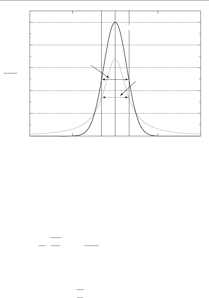
Figure 2.6 shows the two extremes that one may encounter in the absorption lineshape
in atmospheric measurements. These lineshapes are Doppler and Lorentz. A third
lineshape not shown in Figure 2.6 (Voigt) will also be considered in this chapter. The
lineshape factor describes how the vibrational-rotational spectral line intensities of the
previous section are distributed with frequency. In this figure and the following equations,
the maximum lineshape factor
0
occurs at line centre for the three distributions that
will be discussed, and the symbols
D
,
L
, and
V
, respectively, denote the Doppler,
88 Analytical Techniques for Atmospheric Measurement
1.0
Lorentz profile
2
γ
L
2γ
D
0.8
0.6
0.4
0.2
0.0
–0.02 –0.01 0.00
Frequency (ν
– ν
0
) cm
–1
0.01 0.02
Γ(ν)
Γ(ν
0
)
D
Doppler profile
Figure 2.6 Doppler and Lorentz profiles for the same integrated intensity and halfwidth values
D
=
L
. Both profiles are normalized to the peak of the Doppler
0
D
at line center. The peak of the
Doppler profile is 1.48 times the peak of the Lorentz profile.
Lorentz, and Voigt distribution halfwidths in cm
−1
at half the maximum line centre
values.
At low pressures (typically less than 1 torr), the random thermal motions of the
molecules follow a Maxwell–Boltzmann velocity distribution, resulting in a Gaussian
absorption lineshape whose frequency intensity distribution in cm units is given by
the following:
D
cm =
1
D
ln 2
exp
−
−
0
D
2
ln 2
(2.13)
The pre-exponential term is the peak line centre value
0
D
. Equation 2.13 is the general
form of the Gaussian distribution with an integrated value of 1. The Doppler halfwidth
is related to the molecular weight M and temperature T (K) of the gas by:
D
cm
−1
= 3581 ×10
−7
0
T
M
(2.14)
Since IR databases deal with integrated line intensities, while the sensitivity of real-world
instruments typically rely on peak line centre absorptions, it is very useful to integrate
Equation 2.13 (over all frequencies spanning the absorption line) to relate the peak

Infrared Absorption Spectroscopy 89
line centre value to the integrated Doppler linewidth and halfwidth. This results in the
following very useful expression:
0
D
cm =
D
ln 2
=
04697
D
(2.15)
Since most atmospheric trace gas measurements are not carried out using Doppler-
limited pressures, one must also consider two other lineshapes. At high pressures, typically
at several hundred Torr, collisions between molecules dominate the lineshape, which is
described by the following Lorentzian distribution:
cm =
1
L
−
0
2
+
2
L
(2.16)
Here the Lorentz halfwidth
L
cm
−1
at temperature T is related to the broadening
coefficient
0
L
cm
−1
atm
−1
by:
L
T cm
−1
=
0
L
T
0
T
0
T
n
P (2.17)
In this expression, P is the total sample pressure in atm, the exponent n gives the
temperature dependence for the broadening and is typically around 0.5, from simple
collision theory. However, small deviations from this value have been measured or
inferred in many cases. The superscript on the broadening coefficient refers to the
reference temperature T
0
, which usually is 296 or 298 K. Values for
0
L
and n are given
for various molecules in spectral databases such as HITRAN. It is worth noting that
the temperature dependence for the Lorentz broadening is opposite to that for Doppler
broadening, and the net overall effect of temperature will depend upon the exact Lorentz
and Doppler contributions to the absorption lineshape. As with the Doppler profile, one
can derive the following useful expression that relates the peak line centre Lorentz value
0
to the integrated value and halfwidth:
0
cm =
1
L
(2.18)
A comparison of the peak line centre values for the Doppler and Lorentzian profiles
of Equations 2.15 and 2.18 indicates that the Doppler profile yields an absorption 1.48
times larger than the Lorentz profile for equivalent line halfwidths (i.e. a pressure where
L
=
D
). This result is shown in Figure 2.6. One should keep in mind that this is a special
case at a unique sampling pressure for illustrative purposes, only to show the comparison
of the two functions. At such a sampling pressure one cannot simply choose to operate
on one function or the other, since both functions become important in describing the
lineshape, as will now be discussed.
At intermediate sampling pressures of approximately several torr to ∼100 torr (the
exact range of which depends upon the particular molecule and the values of
D
and
L
), both Doppler and Lorentz lineshapes contribute to the overall lineshape, and results
in a new function described by a Voigt function. Since in atmospheric studies most

90 Analytical Techniques for Atmospheric Measurement
instruments operate in this pressure regime, the Voigt function is most frequently the
function of interest. The reader is referred to Mitchell and Zemansky (1961) and Penner
(1959) for some of the original discussions of the Voigt profile and to Armstrong (1967)
and Humlicek (1982) for more discussions and solutions. The Voigt profile is generated
by the convolution of the Doppler and Lorentzian lineshape functions above. In such
a convolution process, one assumes that the two lineshape functions are independent
of one another, and that the new function is generated from the integral of sliding one
function across the other over the entire absorption line (i.e. limits of the integral from
− to +). The convolution process results in the following expression:
cm =
0
D
⎡
⎣
y
−
e
−t
2
y
2
+x −t
2
dt
⎤
⎦
(2.19a)
with
x =
−
0
D
√
ln 2y=
L
D
√
ln 2t=
D
√
ln 2 (2.19b)
The parameter , which is incorporated in the parameter of integration t, is used to
express the Doppler and Lorentz frequency differences during the convolution process
in terms of a single variable. This convolution is carried out by keeping one function
fixed at a value of x and sliding the other function across in cm
−1
steps over the entire
line. The function of Equation 2.19a shows that the Voigt profile can be described by a
unitless fraction (the term in the brackets) times the peak line centre Doppler function,
0
D
. This fraction approaches 1.0 at low pressures (Doppler profile) and takes on values
of 0.02 and lower at high pressures (Lorentz profile), depending upon the broadening
coefficient and the pressure.
The frequency dependence of the various spectral line intensity profiles just introduced
can be related to the integrated spectral line intensity S of the previous section through
the following:
S = S (2.20a)
S
0
=
0
S (2.20b)
Since the shape factor has the unit of cm, the unit of S becomes cm
2
molecule
−1
.
Unfortunately, unlike the Doppler and Lorentz functions, there is no simple relationship
between the integrated and peak Voigt functional values. One must solve Equation 2.19
explicitly for each molecule at the sampling pressures and temperatures employed. This
is not a problem since Equation 2.19 was derived in such a manner as to approximate the
real part of the complex probability function, for which there are a number of efficient
polynomial expansion solutions (Humlicek, 1982 and Armstrong, 1967, to name a few).
Efficient computer code can thus be written to routinely solve the Voigt function under
different conditions. However, one can also solve Equation 2.19 numerically using a
simple spreadsheet program, and it is very instructive to do so for one set of conditions
at the line centre, as shown by the following example.

Infrared Absorption Spectroscopy 91
Example 1
Conditions for example
Gas is CH
2
O, M =30026 g mole
−1
T =296 KP = 500torr = 00658atm
0
= 28316417 cm
−1
(from HITRAN)
S = 504×10
−20
cm
2
cm
−1
molecule
−1
at 296 K (from HITRAN)
L
= 0108 cm
−1
atm
−1
at 296 K from HITRAN)
∗
00658 atm =00071 cm
−1
D
= 00032 cm
−1
(Equation 2.14)
y = 1858 (Equation 2.19b)
x =0 (Equation 2.19b, for the Voigt value at line centre where =
0
)
Range of convolution =±005 cm
−1
over the line, number of steps in convo-
lution = 1000
Resolution of convolution = 01cm
−1
in 1000 steps = 1 ×10
−4
cm
−1
step
−1
Steps in convolution
(1) Calculate values of t and ultimately the entire term in the integral of
Equation 2.19a for each cm
−1
step in sliding one function over the other. We
start at a value =−005cm
−1
, and t becomes −13072.
(2) Calculate e
−t
2
and ultimately the integrand of Equation 2.19a, which results
in negligibly small values of 62 ×10
−75
and 36 ×10
−77
, respectively, for this
particular convolution step.
(3) Repeat this procedure for each of the 1000 steps in the convolution and store
the resultant value of the integrand each time. At line centre where is 0, we
calculate a value of 0.2898 for the integrand.
(4) Integrate all the above individual determinations using a trapezoidal approach,
where the average value of two adjacent determinations is multiplied by the
step size and summed over all the steps.
(5) Multiply the integral by y/ =0591 to arrive at a value of 0.272. The Voigt line
centre value is thus 27.2% of the peak of the Doppler profile. After multiplying
by the Doppler peak 743 ×10
−18
cm
2
molecule
−1
one arrives at a final Voigt
line centre spectral intensity of 202 ×10
−18
cm
2
molecule
−1
.
(6) One can repeat the entire procedure using a different value for v in the function
x to determine the Voigt function at some other frequency.
Figure 2.7(a) shows the results of calculating T = 296 K the Voigt function at line
centre for three different molecules. Both methods of calculation (the simple spreadsheet
method in Example 1 or the Humlicek (1982) polynomial expansion) yield the same
results. In each case we plot the individual Voigt results for the molecule in question
normalized to its specific Doppler value at line centre,
0
V
/
0
D
(this is the fractional
term in the brackets of Equation 2.19a). The main plot shows the relationship as a