Gubbins D., Herrero-Bervera E. Encyclopedia of Geomagnetism and Paleomagnetism

Подождите немного. Документ загружается.

where d l is an element of arc length along C and z

and z

denote the

z -coordinates (parallel to the rotation axis) along, respectively, the top

and botto m geostrophic contours. Neglecting the inertial term on the

LHS, the RHS gives a generalized version of Taylor ’ s condition

(q.v.). The magnetic force j  B gives the term that generates torsional

oscillations ( q.v.) in reaction to the shearing of the magnetic field lines

by the geostr ophic motions. It can be shown that Eq. (2) governs the

time changes of the kinetic energy of the geostrophic motions, in a

frame rotating with the mantle. With spherical boundaries, Eq. (2)

can be interpreted also as the equation governing the transport of angu-

lar momentum within the fluid outer core and the exchanges with the

inner core and the mantle. In presence of topography on the boundaries,

Eq. (2) does not, however, give directly the transport of angular momen-

tum (Fearn and Proctor, 1992). This constitutes, arguably, the main dif-

ficulty of the studies of topographic core-mantle couplin g.

If the solid boundaries were spherical and electrically insulating,

core angular momentum would be conserved and the net torque on

the core would be zero. This is obviously true but this may also be

directly inferred from Eq. (2). Taking into account topography and

using a perturbation approach, only the s and z components of the

magnetic and buoyancy forces are involve d in the terms that are

dependent (linearly) on the topography on the RHS of Eq. (2), while a

spherical approximation can be used on the LHS. The constraint of con-

servation of core angular momentum carried by geostrophic motions

does not apply any more.

Taking for the sake of the demonstration insulating solid boundaries

in a core model, the only torque left to modify the total core angular

momentum is the pressure torque G

. Indeed, the buoyancy and mag-

netic forces that accelerate the geostrophic motions within the core

are unable to account for the exchanges of angular momen tum with

the mantle. Conversely, when there is a nonzero pressure torque, there

are time changes of u

and Taylor’ s condition is not exactly obeyed.

Thus, in an average state, fulfilling Taylor’s condition, the pressure

torque would vanish. In the actual Earth, the different contributions

to Eq. (1) probably tend to cancel out also except if the electromag-

netic torque acting between core and mantle is strong enough to

oppose G

. This explains why it will be difficult to estimate G

from

geophysical data. If such a cancelation does not take place and if the

height of the topography is of the order of 1 km, the pressure torque

is much larger than the torque responsible for the observed changes

in the Earth ’ s rotation (Jault and Le Mouël, 1990).

From a theoretical viewpoint, it may not be possible to study sepa-

rately the different torques acting between core and mantle. As an

example, addition of a conducting layer at the bottom of the mantle

to the model and inclusion of CMB topography cannot be considered

in isolation. Both modify the RHS of Eq. (2). Kuang and Chao (2001,

2003) have adapted a numerical geodynamo model to study topo-

graphic coupling. Their solutions are calculated in a spherical shell

with boundary conditions modified to mimic the role of the CMB

topography. With this approach, the main ingredient of topographic

coupling, distortion of the geostr ophic contours, is included. Kuang

and Chao have verified that, in their model, the different contributions

to the pressure torque tend to cancel out.

Role of the inner core

The main pressure torque acting on the fluid outer core may result

from the action of the hydro static pressure on the ICB topography if

the ICB does not coincide with an equipotential surface of the gravity

field. It is unimportant for the outer core since it cancels exactly a

gravity torque acting from the mantle on the outer core. On the other

hand, pressure and gravity torques acting on the inner core do not can-

cel out (see Inner core oscillation; Inner core, rotational dynamics).

Differential rotation between the inner core and the mantle may have

some influence on topographic core-mantle coupling because it entails

time changes of the geometry of geostrophic contours.

If the height of the topography either on the ICB or on the CMB is not

negligible, the cylinder tangent to the inner core equator is not of constant

height. Then, there are regions void of closed contours separated by con-

stant height on both sides of the tangent cylinder. There, the role of the

geostrophic motions is taken over by low-frequency z-independent inertial

waves, known as Rossby waves (Greenspan, 1968, pp. 85–90).

Perspectives

Hopefully, understanding of core-mantle coupling will result from on-

going studies of the propagation of torsional waves within the fluid outer

core. Considering the pressure acting on the mantle suffices to calculate

the net torque on the mantle but not to estimate how CMB and ICB topo-

graphies influence the distribution of geostrophic velocity within the

core. Knowledge of the volume forces is required, except in the special

case of distortion of the geostrophic contours in the z-direction only,

which happens when topography is antisymmetrical with respect to the

equatorial plane (Jault et al., 1996). Topographical effects have not yet

been adequately taken into account in models of torsional waves.

Perhaps, too much weight has been given in this entry on Taylor’s

condition. Rapid changes in the differential rotation between geos-

trophic cylinders are definitely opposed by magnetic forces within

the core. On the other hand, only viscous coupling and magnetic cou-

pling with the weakly conducting mantle control global oscillations of

the fluid outer core with respect to the mantle.

Dominique Jault

Bibliography

Bell, P.I., and Soward, A.M., 1996. The influence of surface topography

on rotating convection. Journal of Fluid Mechanics, 313:147–180.

Fearn, D.R., and Proctor, M.R.E., 1992. Magnetostrophic balance in

nonaxisymmetric, nonstandard dynamo models. Geophysical and

Astrophysical Fluid Dynamics, 67:117–128.

Greenspan, H.P., 1968. The Theory of Rotating Fluids. Cambridge:

Cambridge University Press.

Hide, R., 1969. Interaction between the Earth’s liquid core and solid

mantle. Nature, 222: 1055–1056.

Hide, R., 1977. Towards a theory of irregular variations in the length

of the day and core-mantle coupling. Philosophical Transactions

of the Royal Society, 284: 547–554.

Jault, D., and Le Mouël, J.-L., 1990. Core-mantle boundary shape:

constraints inferred from the pressure torque acting between the core

and mantle. Geophysical Journal International, 101: 233–241.

Jault, D., Hulot, G., and Le Mouël, J.-L., 1996. Mechanical core-

mantle coupling and dynamo modelling. Physics of the Earth and

Planetary Interiors, 98: 187–191.

Kuang, W., and Chao, B.F., 2001. Topographic core-mantle coupling in

geodynamo modeling. Geophysical Research Letters, 28:1871–1874.

Kuang, W., and Chao, B.F., 2003: Geodynamo modeling and core-

mantle interactions. In Dehant, V., Creager, K., Karato, S.-I., and

Zatman, S. (eds.), Earth’s Core Dynamics, Structure, Rotation.

Washington, DC: American Geophysical Union, pp. 193–212.

Cross-references

Core-Mantle Boundary Topography, Implications for Dynamics

Core-Mantle Boundary Topography, Seismology

Core-Mantle Coupling, Electromagnetic

Inner Core Oscillation

Inner Core Tangent Cylinder

Inner Core, Rotational Dynamics

Length of Day Variations, Decadal

Oscillations, Torsional

Taylor’s Condition

136 CORE-MANTLE COUPLING, TOPOGRAPHIC

COWLING, THOMAS GEORGE (1906–1990)

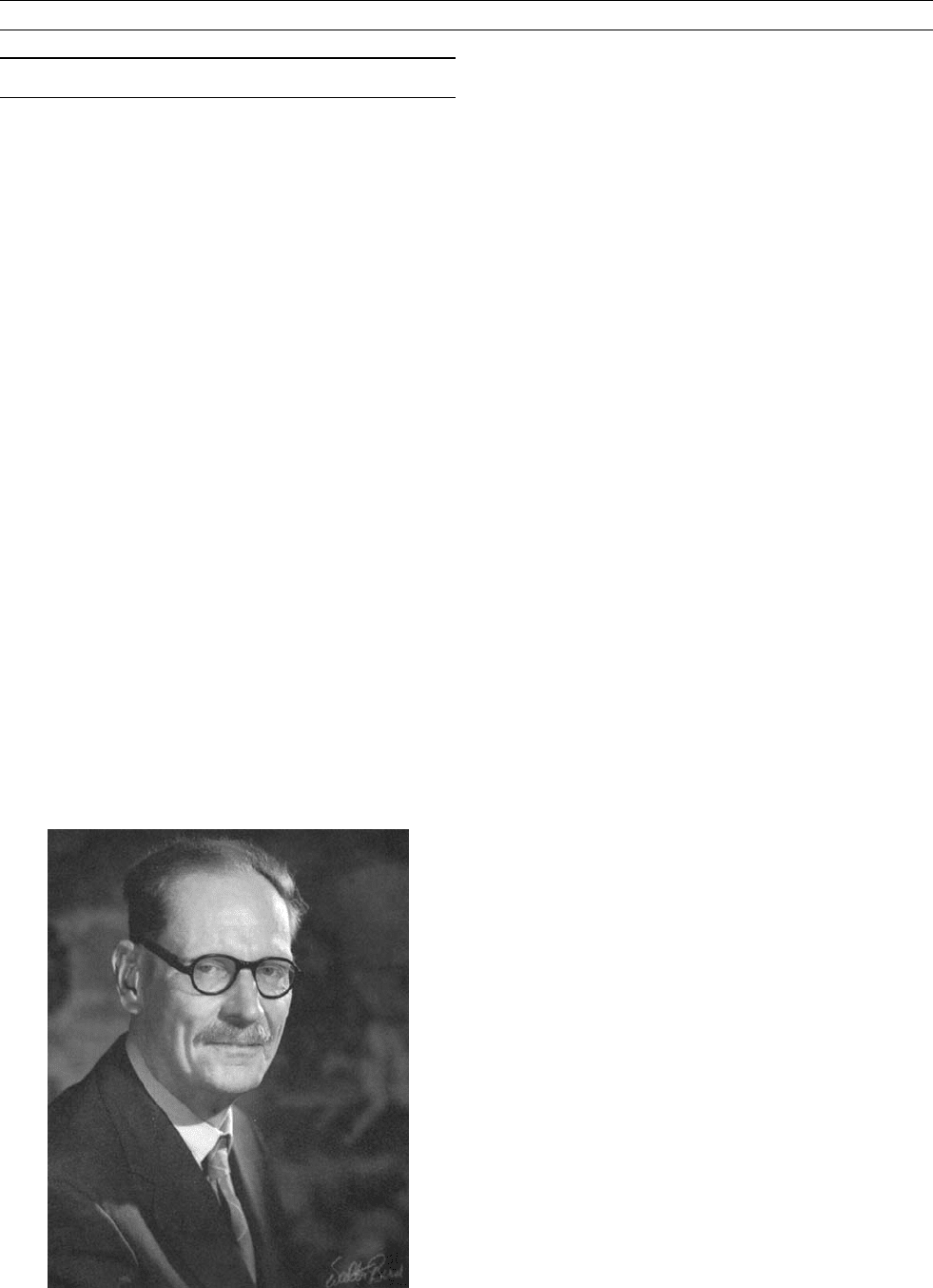
Thomas George Cowling (Figure C45), applied mathematician and

astrophysicist, was born on June 17, 1906 at Hackney, London, the

second of the four sons of George Cowling, post office engineer,

and Edith Eliza Cowling (née Nicholls). His grandparents and their

antecedents were nearly all artisans, blue-collar workers, servants, or

sailors. Tom was educated at Sir George Monoux Grammar School,

from where in 1924 he won an open scholarship in mathematics to

Brasenose College, Oxford. He won the University Junior Mathematical

Exhibition in 1925 and the Scholarship in 1926. A first class degree was

rewarded by a three-year post-graduate scholarship at Brasenose, his

research supervisor being the cosmologist Edward A. Milne.

Cowling’s acumen was quickly recognized. After gaining his

D.Phil., he went by invitation to join Sydney Chapman (q.v.)at

Imperial College as demonstrator. Their collaboration converted

Chapman’s “skeleton” of a book into a standard text, The Mathemati-

cal Theory of Non-Uniform Gases (1939), which treats kinetic theory

by a systematic attack on the classical Boltzmann equation. Cowling

was subsequently assistant lecturer in mathematics at Swansea (1933–

1937), and lecturer at Dundee (1937–1938) and at Manchester

(1938–1945). From 1945–1948 he was professor of mathematics at

Bangor, moving then to his last post as professor of applied mathe-

matics at Leeds, becoming emeritus professor in 1970.

Over the three decades 1928–1958, Cowling made outstanding con-

tributions to stellar structure, cosmical electrodynamics, kinetic theory

and plasma physics. Recognition came with the Johnson Memorial

Prize at Oxford (1935), election to the Royal Society (1947), the Gold

Medal of the Royal Astronomical Society (1956) and its presidency

(1965–1967), Honorary Fellowship of Brasenose (1966), the Bruce

Medal of the Astronomical Society of the Pacific (1985), and the

Hughes Medal of the Royal Society (1990).

Tom Cowling married Doris Marjorie Moffatt on August 24, 1935.

There were three children: Margaret Ann Morrison, Elizabeth Mary

Offord (deceased 1994), and Michael John Cowling, and six grand-

children.

A few years before Cowling began working on stellar structure, Sir

Arthur Eddington had published his celebrated Internal Constitution of

the Stars, in which he pictured a homogeneous star as a self-gravitat-

ing gaseous sphere in radiative equilibrium, with its luminosity fixed

by its mass and chemical composition. From comparison of his “stan-

dard model” with the masses and radii of observed “main-sequence”

stars, Eddington inferred that the as yet unknown stellar energy

sources must be highly temperature-sensitive. Cowling’s careful analy-

sis strengthened Eddington’s case—against the criticisms of Sir James

Jeans—by showing that the models would nevertheless almost cer-

tainly be vibrationally stable. In parallel with Ludwig Biermann, he

also showed that a stellar domain that satisfies the Schwarzschild

criterion for convective instability and becomes turbulent needs only

a very slightly superadiabatic temperature gradient in order to convect

energy of the order of a stellar luminosity.

The “Cowling model,” with its nearly adiabatic convective core,

surrounded by a radiative envelope, is a paradigm for stars somewhat

more massive than the Sun, for which energy release by fusion of

hydrogen into helium takes place through the highly temperature-

sensitive Bethe-Weizsäcker carbon -nitrogen cycle. In low-mass stars

like the Sun, hydrogen fusion occurs via the much less temperature-

sensitive proton-proton chain, so that the energy-generating core is

now radiative; but because of the low surface temperature, there is a

deep convective envelope, extending from just beneath the radiating

surface. Biermann’s calculated depth for the solar convection zone

has been confirmed by helioseismology. Biermann also showed that

a star of ’ M



=4 would be fully convective. Cowling pointed out

that for these stars, the luminosity must still satisfy the condition of

radiative transport through the nonconvecting surface layers. Earlier,

Milne had argued that the luminosity of all stars should be sensitive to

conditions in the surface, rather than depending essentially on radiative

transfer through the bulk of the star, as in Eddington’s theory. Cowling’s

work vindicated Eddington’s approach for main-sequence stars, while

implicitly allowing for such sensitivity in giant stars and pre-main

sequence stars, with extensive sub-surface convective zones.

Cowling’s other contributions to stellar structure include an impor-

tant paper on binary stars, and two pioneering papers on nonradial stel-

lar oscillations, foreshadowing today’s work in helioseismology.

Simultaneous with his work on stellar structure, Cowling published

a series of studies on cosmical magnetism and on plasma physics, cul-

minating in his superbly succinct monograph Magnetohydrodynamics

(1959, 1976). Together with Biermann, Arnulf Schlüter, and Lyman

Spitzer Jr., he did much to clarify the concept of “conductivity” for

both fully and partially ionized gases. A lively correspondence with

Biermann in the 1930s brought out the requirements of a theory of

both the structure and the origin of sunspots, and indeed may be

thought of as the genesis of the study of magnetoconvection. While

recognizing the seminal contributions of Hannes Alfvén (q.v.) to cos-

mical magnetism (“Alfvén’s best ideas are very good indeed”), he

had earlier applied his renowned critical faculties to a demolition of

Alfvén’s theory of the sunspot cycle and defended the pioneering

Chapman-Ferraro, quasi-MHD theory of geomagnetic storms against

what he regarded as unjust attacks.

In the geomagnetic and in fact in the general scientific world,

Cowling is probably best known for his “antidynamo theorem” (see

Cowling’s Theorem). Sir Joseph Larmor (q.v.) had suggested that

motion of the conducting gas across a sunspot magnetic field yields

an emf, which drives currents against the Ohmic resistance, and these

currents could be just those required by Ampère ’s law to maintain the

assumed field. Cowling began what he expected to be a “relatively

routine piece of difficult computation,” to see what sort of field could

be maintained by the Larmor process. He found instead that for an

axisymmetric field, the required condition breaks down at the ring of

neutral points. In the absence of an energy supply, the Ohmic decay

of the axisymmetric field can be pictured as the steady diffusion of

closed field lines into the neutral point. The moving gas drags field

lines around meridian planes, but does not generate new ones to

replace the disappearing loops—that would require gas to emerge

from the neutral point with infinite speed. This qualitative argument

Figure C45 Thomas George Cowling.

COWLING, THOMAS GEORGE (1906–1990) 137

can be generalized to apply to fields that are topologically similar to

the axisymmetric fields.

For a while, Cowling does seem to have surmised that there was

waiting to be proved a much more general antidyn amo theorem. Later

he felt that too much emphasis was laid on his and other antidynamo

theorems: their significance is that those fields that can be dynamo-

maintained cannot be simple in structure or in mathematical formula-

tion. He illustrated this by showing how one prima facie convincing

general algorithm, designed for the construction of the velocity field

that will maintain a prescribed magnetic field, when applied to a field

which is known to be ruled out by an anti-dynamo theorem yields —

unsurprisingly —“velocities ” that are pure imaginary. He appears to

have provisionally accepted the now familiar picture by which nonuni-

form rotation acting on a given poloidal field generates a toroidal field,

which in turn yields the required new poloidal flux when acted upon

by nonaxisymmetric convective motions —the “ a-effect” in current

dynamo terminology. While remaining well aware of the lacunae in

our present theoretical knowledge, he concluded (1981): “The dynamo

theory of the Sun ’s magnetic field is subject to a number of unresolved

objections, but alternative theories advanced so far are open to much

greater objections. ”

In the absence of dynamo action, the high conductivity of stellar

plasma yields an Ohmic decay time for a large-scale primeval

stellar field that can exceed the lifetime of the star. This “ fossil ” field

picture is inapplicable to the Sun, in which the poloidal field is

now known to reverse as part of the solar cycle, but it remains relevant

to the observed strongly magnetic stars, convincingly modelled as

oblique magnetic rotators. However, for the Earth, the much smaller

length scales yield a decay time that is far too short, so that for both

the Sun and the Earth, dynamo maintenance appears to be mandatory.

In his autobiographical essay “Astronomer by accident ” (1985),

Cowling remarks that he and his brothers inherited the “Puritan work

ethic” from their nonconformist parents. He remained an active, non-

fundamentalist Baptist, though in his later years he confessed to

doubts, speaking of “ getting closer to mysticism rather than to a reli-

gion of set creeds. ” His puritanism perhaps showed itself in his very

high academic standards, which he applied as much to his own work

as to that of others, and earned him the nickname “Doubting Thomas. ”

Everyone knew him by sight: his red hair and his great height made

him conspicuous. They also looked up to him metaphorically, because

of his combination of kindliness and intellectual power.

Cowling ’ s research activity in his later decades was severely ham-

pered by recurring bouts of ill-health, beginning with a duodenal ulcer

in 1954. He died in Newton Green Hospital, Leeds on June 15, 1990.

Leon Mestel

Bibliogr aph y

Chapman, S., Cowling, T.G., 1939. The Mathematical Theory of Non-

Uniform Gases. 1991 Paperback edition. Cambridge: Cambridge

University Press.

Cowling, T.G., 1957. Magnetohydrodynamics . Interscience (2nd ed.,

1976, Adam Hilger).

Cowling, T.G., 1981. The present status of dynamo theory. Annual

Review of Astronomy and Astrophysics, 19:115–135.

Cowling, T.G., 1985. Astronomer by accident. Annual Review of

Astronomy and Astrophysics, 23:1–18.

Mestel, L., 1991. Thomas George Cowling. Biographical Memoirs of

Fellows of the Royal Society, 37 : 103 –125.

Cross- refere nces

Alfvén, Hannes Olof Gösta (1908 –1995)

Chapman, Sydney (1888 – 1970)

Cowling ’s Theorem

Lamor, Joseph (1857 –1942)

COWLING’S THEOREM

Among the theorems of applied mathematics Cowling ’s theorem on

the impossibility of axisymmetric homogeneous dynamos has played

a special role because it has cast in doubt for 40 years the dynamo

hypothesis of the origin of geomagnetism. This hypothesis goes back

to Larmor (1919; see Larmor, J. ) who argued that the magnetic field

of sunspots could be created by motions in an electrically conducting

fluid. He envisioned an axisymmetric model where radial motion into

a cylindrical tube of magnetic flux would cause an electromotive force

v  B driving an electric current in the azimu thal direction, which in

turn would enhance the magnetic flux in the cylinder. While this

model appears to be superficially convincing, Cowling was able to

prove that such a dynamo process is not possible.

The proof originally provided by Cowling (1934 ; see Cowling, T.G.)

is quite simple since he was only concerned with the possibility of the

steady generation of a field confined to meridional planes as envi-

sioned by Larmor. A general axisymmetric magnetic field B satisfying

the condition r B ¼ 0 can be described by

B ¼rA

 e

þ B

(Eq. 1)

where e

is the unit vector in the azimuthal directi on and A

is the

f -component of the magnetic vector potential A . Ohm ’s law for an

electrically conducting fluid moving with the velocity field v can be

written in the form

lrB ¼ v  B rU 

]

] t

A (Eq. 2)

where the last two terms represent the electric field and where the

magnetic diffusivity l is the inverse of the product of magnetic perme-

ability and electrical conductivity of the fluid, l ¼ðs  mÞ

 1

. Since we

are considering an axisymmetric steady process ð] = ] t Þ A vanishes and

r U does not contribute to the f -component of Eq. (2). The latter

assumes the form

]

] r

C þ v

]

] z

C ¼ l

]

] r

C þ

]

] z

C 

]

] r



(Eq. 3)

where a cylindrical coordinate system ðr ; f ; z Þ has been used and

C ð r ; zÞ rA

has been introduced after multiplication of the equation

by r. The condition that the magnetic field is generated locally requires

that it decays towards infinity at least like a dipolar field, i.e., in pro-

portion to ð r

þ z

 3=2

. The function C (r, z ) thus must decay at least

like ðr

þ z

1= 2

. Since, on the other hand, C vanishes on the axis,

r ¼ 0, it must assume at least one maximum or minimum at a point

, z

) at which ð]=]rÞC ¼ð] =]zÞC ¼ 0 can be assumed. Such a point

in the meridional plane is sometimes called “neutral line.” Because at a

maximum or minimum usually ð]

= ] r

ÞC þð]

= ] z

Þ C 6¼ 0 holds, a

contradiction to Eq. (3) is obtained. In the case of “flat ” maxima

or minima where ð]

=]r

ÞC þð]

=]z

ÞC may vanish a similar contra-

diction can be constructed, but this requires a more technical approach.

It should be noted that the above argument does not require a

solenoidal velocity field, rv ¼ 0, as Cowling had originally

assumed. For a generalization of Cowling’s original theorem, which

emphasizes its topological nature, see Bullard (1955; see Bullard, E. C.).

Backus and Chandrasekhar (1956) later refined Cowling’sproofby

eliminating the possibility of an axisymmetric dynamo with a finite

component B

For geophysical and astrophysical applications it is important to

consider the possibility of axisymmetric dynamos caused by varying

magnetic diffusivity or by time-dependent processes. The former pos-

sibility was eliminated by Lortz (1968) while the latter problem moti-

vated Braginsky (1964) to seek a new mathematical approach based on

energy arguments. Braginsky also introduced the spatial configuration

138 COWLING’S THEOREM

of a finite axisymmetric domain V of constant electrical conductivity

surrounded by an insulating space outside. For his proof of the impos-

sibility of time-dependent axisymmetric dynamos he had however to

assume a solenoidal velocity field. For the domain V, Hide (1979)

introduced as a new definition for a dynamo that the magnetic flux

intersecting the surface ]V of V remains finite as the time t tends to

infinity,

jB  d

Sj 6! 0 for t !1: (Eq. 4)

Hide and Palmer (1982) tried to prove on this basis Cowling’s theorem

under rather general conditions. In view of their novel approach it is

unfortunate that their proof turned out to be incomplete (Ivers and

James, 1984; Núñez, 1996). The efforts of Lortz and coworkers were

thus required to arrive at mathematically rigorous conclusions about

the impossibility of the generation of axisymmetric magnetic field by

time dependent and not necessarily solenoidal velocity fields. For

references and details of the mathematical issues we refer to the

reviews of Ivers and James (1984) and Núñez (1996).

Cowling (1955) had already realized that the ideas of the proof for

the impossibility of an axisymmetric dynamo could easily be applied

to prove the impossibility of two-dimensional dynamos for which

the magnetic field depends only on two of the three coordinates of a

cartesian system. Since the cartesian case is somewhat simpler to deal

with many of the mathematical problems have first been explored in

this geometry. The 1955 Cowling paper is particularly important in

its showing that—because of the presence of non-Hermitian opera-

tors—the apparently general kinematic dynamo formalism developed

by Elsasser (1947 and earlier papers referred therein; see Elsasser, W.)

does not guarantee real valued velocities. Cowling illustrates this

by showing that the two-dimensional model yields purely imaginary

velocities.

It is of interest to note that dynamos with small deviations from axi-

symmetry can readily be realized. The theory of spherical dynamos

developed by Braginsky (1976; see Dynamo, Braginsky) is based

on a small perturbation of an axisymmetric configuration. A purely

axisymmetric dynamo has been obtained by Lortz (1989) by allow-

ing for a small anisotropy of the magnetic diffusivity tensor. It thus

appears that in spite of its early negative influence Cowling ’s theorem

has stimulated the understanding of dynamo action and the creation of

ingenious solutions for the problem of magnetic field generation.

Friedrich Busse

Bibliography

Backus, G., Chandrasekhar, S., 1956. On Cowling’s theorem on the

impossibility of self-maintained axisymmetric homogeneous

dynamos. Proceedings of the National Academy of Sciences, 42:

105–109.

Braginsky, S.I., 1964. Self-excitation of a magnetic field during the

motion of a highly conducting fluid. Soviet Physics JETP., 20:

726–735.

Braginsky, S.I., 1976. On the nearly axially-symmetrical model of

the hydromagnetic dynamo of the Earth. Physics of the Earth

and Planetary Interiors, 11: 191–199.

Bullard, E., 1955. A discussion on magneto-hydrodynamics: Intro-

duction. Proceedings of the Royal Society of London , A233:

289–296.

Cowling, T.G., 1934. The magnetic field of sunspots. Monthly Notices

of the Royal Astronomical Society, 34:39–48.

Cowling, T.G., 1955. Dynamo theories of cosmic magnetic fields. Vis-

tas in Astronomy, 1: 313–323.

Elsasser, W.M., 1947. Induction effects in terrestrial magnetism, Part

III Electric modes. Physical Review, 72: 821–833.

Hide, R., 1979. On the magnetic flux linkage of an electrically-

conducting fluid. Geophysical and Astrophysical Fluid Dynamics,

12: 171–176.

Hide, R., Palmer, T.N., 1982. Generalization of Cowling’s theorem.

Geophysical and Astrophysical Fluid Dynamics, 19: 301–309.

Ivers, D.J., James, R.W., 1984. Axisymmetric antidynamo theorems in

compressible non-uniform conducting fluids. Philosophical Trans-

actions of the Royal Society of London, A312: 179– 218.

Larmor, J., 1919. How could a rotating body such as the sun become a

magnet? The British Association for the Advancement of Science

Report, 159–160.

Lortz, D., 1968. Impossibility of steady dynamos with certain symme-

tries. Physics of Fluids, 10

: 913–915.

Lortz, D., 1989. Axisymmetric dynamo solutions. Zeitschrift für Nat-

urforschung, 44a: 1041–1045.

Núñez, M., 1996. The decay of axisymmetric magnetic fields:

A review of Cowling’s theorem. SIAM Review, 38: 553–564.

Cross-references

Bullard, Edward Crisp (1907–1980)

Cowling, Thomas George (1906–1990)

Dynamo, Braginsky

Elsasser, Walter M. (?–1991)

Larmor, Joseph (1857–1942)

COX, ALLAN V. (1926–1987)

Allan Cox was one of the preeminent geophysicists of his generation.

He made many important scientific contributions to the field of paleo-

magnetism and to the study of plate tectonics. His untimely death at

the age of 61 was a loss to Stanford University, his home institution,

and to the geophysics community.

Cox was born in Santa Ana, California, in 1926 as the son of a

house painter. He attended the University of California at Berkeley

where he started his education as a chemistry major. He only went to

Berkeley for one quarter before he dropped out and joined the mer-

chant marine. His work in the merchant marine allowed him time for

one of his great loves, reading over a wide range of topics. After three

years in the merchant marine, he returned to Berkeley, again as a

chemistry major. One of his life defining experiences at that time

was spending summers in Alaska with geologist Clyde Wahrhaftig of

the U.S. Geological Survey. These summer jobs gave Cox a strong

love of geology. When he returned to Berkeley to continue his educa-

tion at the end of the summer, he found chemistry dull by comparison

and his grades suffered. This led to the loss of his student deferment

from the military draft and he ended up in the army for two years.

When he came back to Berkeley after the army, strongly motivated

to succeed at his studies, he changed his major to geology. In 1955,

he earned his bachelor of arts from Berkeley in geology. He continued

his education with graduate work in geology at Berkeley. His initial

intent was to study ice and rock glaciers, the objects of his summer

field work with Wahrhaftig, but instead he decided to work with John

Verhoogen on rock magnetism. At that time Verhoogen was one of the

few Berkeley faculty members who was receptive to the idea of conti-

nental drift. This gave Cox an early exposure and interest in the field

that would become plate tectonics.

Cox received a master of arts in 1957 and his PhD from Berkeley in

1959 and went to work at the U.S. Geological Survey in Menlo Park,

California. At the Survey he worked with another rock magnetist, Dick

Doell, on the paleomagnetic record of geomagnetic field reversals. For

this work, Cox and Doell needed some way to accurately date the

rocks carrying paleomagnetic records of reversed and normal geomag-

netic field polarity, so they convinced the U.S. Geological Survey to

COX, ALLAN V. (1926–1987) 139

hire Brent Dalrymple who could use the radiogenic decay of K to Ar

to determine the age of igneous rocks being studied paleomagnetically.

The research team of Cox, Doell, and Dalrymple made important

contributions to Earth science by unraveling the record of polarity

intervals of the geomagnetic field over the past 5 Ma. They traveled

to far corners of the globe to collect igneous rocks of various ages,

measured their paleomagnetism at their laboratory in Menlo Park, con-

ducted demagnetization experiments to isolate the primary magnetiza-

tion of the rocks, and dated the rocks radiogenically. There was

spirited competition with other researchers conducting similar research

at this time, particularly an Australian team consisting of Tarling,

Chamalaun, and McDougall, based at the Australian National Univer-

sity. The two teams would make friendly wagers about who would

discover the next polarity interval in the quest for the full revelation

of the geomagnetic polarity time scale. The bets would be paid off,

usually in cocktails, at the next professional meeting. The geomagnetic

timescale for the past 5 Ma was completed by 1969 and was crucial to

the seafloor spreading interpretation of the seafloor magnetic anoma-

lies that were discovered to be parallel to the mid-ocean ridges at about

this time.

In 1967, Allan Cox moved from the U.S. Geological Survey to

nearby Stanford University in Palo Alto, California, and became the

Cecil and Ida Green Professor of Geophysics. At Stanford he studied

various aspects of paleomagnetism with his graduate students, contri-

buting to the understanding of many topics, including the transition

of the geomagnetic field between polarity states, the characteristics

of geomagnetic field intensity, the statistics of polarity interval lengths,

the rock magnetics of seafloor basalts and sedimentary rocks, vertical

axis rotations of tectonic blocks, and the structure of a plate’s apparent

polar wander path. He developed a strong interest in the paleolatitudi-

nal motion of the tectonostratigraphic terranes that were just being

recognized by geologists at that time.

In 1979, he became dean of Stanford’s School of Earth Sciences and

showed a gift for being an administrator. During his stint as dean he

kept up his teaching and his research and stayed involved with under-

graduates, through undergraduate research projects and helping design

the lighting for the student theatre. He was viewed as the paramount

example of a true teacher-scholar, excelling equally at teaching,

research, and service to Stanford University and his professional socie-

ties. He also served his community in the hills to the west of Palo Alto,

studying with fellow faculty members and students the effects of log-

ging on soil erosion and watersheds and publishing a small book on

the subject, Logging in Urban Counties.

Allan Cox had a productive scientific career, publishing over 100

scientific journal articles and two textbooks on plate tectonics, Plate

Tectonics and Geomagnetic Reversals and Plate Tectonics, How it

Works with Robert B. Hart. He also received many professional hon-

ors. He was elected to the National Academy of Sciences, the Ameri-

can Philosophical Society, and the American Academy of the Arts and

Sciences. He was president of the American Geophysical Union from

1978–1980. He received the Day Medal of the Geological Society of

America, the Fleming Medal of the American Geophysical Union,

and the Vetlesen Medal of Columbia University.

He died in a bicycle accident on January 27, 1987, running off the

road in the hills west of Stanford and into a redwood tree. Tragically,

his death was ruled a suicide, probably brought on by failings and

crises in his personal life.

Kenneth P. Kodama

Bibliography

Cox, A.V., 1973. Plate Tectonics and Geomagnetic Reversals. San

Francisco, CA: W.H. Freeman and Company.

Cox, A.V., and Hart, R.B., 1986. Plate Tectonics, How it Works. Palo

Alto, CA: Blackwell Scientific.

Cross-references

Paleomagnetism

Shaw and Microwave Methods, Absolute Paleointensity Determination

CRUSTAL MAGNETIC FIELD

Introduction

Magnetic minerals in the rocks in the upper lithosphere of the Earth and

other differentiated planetary bodies having dynamos generate mag-

netic fields when the minerals are in a cooler environment than their

individual Curie temperatures. These magnetic fields are useful for

studying crustal materials for a variety of applications. The most widely

known example of the utility of the field is its role in deciphering the

process of seafloor spreading through the recognition of alternately nor-

mally and reversely magnetized rock stripes on the ocean floor (see

Magnetic anomalies, marine; Magnetic anomalies for geology and

resources). In continental regions, the use of crustal magnetic field is

well-known to Earth scientists because the short-wavelength part of

the field closely correlates with the near-surface geologic variations.

Crustal magnetic field is thus a proxy for crustal geology and is useful

in understanding the structure and composition of the crust as well as

its evolution especially when surficial sediments and other geologic for-

mations obscure subsurface geology. Readers interested in the details of

the methods on processing, analysis, and interpretation of the entire

spectrum of crustal magnetic fields should consult the books by Blakely

(1995) and Langel and Hinze (1998).

Magnetization is a complex phenomenon and for rocks it is depen-

dent on a variety of conditions the rocks are exposed to—beginning

with their formation, through their tectonic evolution, and exposure

to their surroundings and the ambient conditions. A part of the magne-

tization of the rocks has the memory of these past conditions (based

on the strength and direction of the past magnetic field at the time

when the rocks are formed or chemically altered, its environmental

history/metamorphism, e tc.): this memory is retained as components

known as “remanent magnetization” (see M agnetization, remanent

and Magnetization, natural remanent (NRM)). The present condi-

tions (magnitude and direction of the surrounding ambient magnetic

field, temperature, and mineral chemistry) to which magnetizable

minerals in the rocks are exposed are reflected in their “induced

magnetization.” A vector sum of the induced magnetization a nd

all retained remanent components leads to “total magnetization” of

rocks, which causes the magnetic field in th e neighborhood of the

rocks. This field attenuates with increasing distance from the rocks,

adds to the fields originating from the surrounding ro cks, and

“perturbs” the fields at the observation location caused by the pla-

netary dynamo, electrical c urrents i n the ionosphere and the m agne-

tosphere (the external fields), and induction due to conductivity

structure o f the planetary interior (see Core, electrical conductivity

and Mantle, electrical conductivity, mineralogy). The perturbing

field is traditionally called the “anomalous” field and this is the

crustal magnetic field.

The field of the planetary dynamo and the external fields vary

spatially as well as in time (see Geomagnetic secular variation and

Geomagnetic spectrum, spatial), and models estimating them at the

location and time of observations are required to extract the crustal

magnetic field from the raw magnetic field observations. Because the

conductivity structure of the Earth is not well-known, its contribution

is customarily not explicitly removed when deriving the crustal mag-

netic field, but efforts are underway to estimate and remove the non-

magnetization-related effects from the observed magnetic field in

areas where the conductivity variation is large and the geometry is

known (e.g., ocean-continent conductivity contrast; see Coast effect

140 CRUSTAL MAGNETIC FIELD

of induced currents). The typical model describing the core-field

dynamo is called the International Geomagnetic Reference Field

(IGRF) (q.v.). However, this does not include the external fields and,

therefore, stationary magnetometer basestations tracking the time var-

iations of the external field are employed in a local region of surveys

(see Aeromagnetic surveying); these time-varying external fields

are then removed from the survey observations to construct the mag-

netic anomaly field. To reduce the effects of imperfect and incomplete

reference models and any remaining inconsistencies in the derived

anomaly field, it is typical to perform surveys with tracks crossing

each other (also called tie-lines) so that the anomaly mismatches at

the cross-over locations could be minimized subject to assumptions

regarding the nature of the spatiotemporal variations of the external

field and the induction effects in the region. Deployment of base sta-

tions is not always feasible where surveys are made along tracks

longer than a few hundred kilometers (typically over the oceans,

but also for continental surveys designed for the determination of

the long-wavelength anomaly field). A recently developed specialized

model, known as the comprehensive model (CM) (Sabaka et al.,

2002), is useful to estimate and remove these noncrustal magnetic field

components from such regional survey data. The CM describes the

core field and its variation, the long-wavelength variation of the exter-

nal fields during the magnetically quiet periods, and the first-order

induced fields in the Earth using the permanent observatory records

beginning 1960s, augmented by fields measured by satellites to fill

the large spatial gaps in the magnetic observatory coverage in many

parts of the world. Since the CM is a temporally continuous model

in comparison to the piece-wise continuous IGRF, it is also effective

in minimizing survey base-level mismatches noticeable when neigh-

boring surveys are combined (see examples in Ravat et al., 2003).

On Earth, in the near-surface environment, crustal field generally

has magnitude range of a few hundred nanoteslas (nT, an SI unit

of magnetic field strength) — much smaller compared to the core-

generated magnetic field of 24000–65000 nT (see Main field maps).

However, over magnetically rich iron formations the magnitude

of the crustal field above the Earth’s surface can exceed 10000 nT

regionally, for wavelengths of a few hundreds of kilometers (e.g., Kursk

iron formations in Ukraine). Locally, the magnitude of the anomalies

can be stupendously large: for example, ground magnetic surveys over

parts of Bjerkreim-Sokndal layered intrusion in Rogaland, Norway,

where hemo-ilmenitic rocks having remanent magnetization up to

74 A/m have been measured, a nearly 30000 nT anomaly trough spans

the distance of only 500 m (McEnroe et al., 2004). In such places, even

compass needles are rendered useless in their usual magnetic north-

pointing purpose because they are attracted by the magnetism of the

neighboring rocks rather than the Earth’s core-generated magnetic field.

The sensitivity of commonly available field magnetometers is better

than 0.1 nT (see Aeromagnetic surveying) and the relative precision of

the measurement (which depends partly also on the relative precision

of spatial coordinates and the time of measurements) nearly approaches

this number in carefully executed surveys. Thus, it is possible to resolve

reliably very small spatial changes in magnetic field especially over

elongated geologic sources (e.g., dikes or faults). Thus, a magnetic

map consists of patterns associated with geology and can be interpreted

with fractal magnetization and pattern recognition/characterization

concepts (e.g., Pilkington and Todoeschuck, 1993, in Blakely, 1995;

Maus and Dimri, 1994; Keating, 1995); this is discussed further in the

interpretation methods section.

Examples of the utility of the field

How the crustal magnetic field is used by Earth scientists and the

superb subsurface detail reflected in it are best conveyed using simple

visual correlations of high-resolution magnetic and geologic maps.

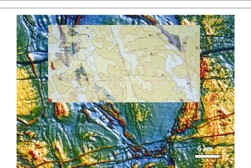
Figure C46/Plate 7c shows such a map from the poorly exposed Arch-

ean age province of western Australian cratons under the Precambrian

and recent cover rocks. In the figure, the magnetic map is superim-

posed partly by the geological map prepared by Geological Survey

of Western Australia and Geoscience Australia from surface outcrops

and mining information. Considerable gold workings have been

developed in the greenstone formations that form the linear magnetic

highs in the shape of an ovoid in the center of the map (this structure

is common when domal uplifts have been partly eroded). Aeromag-

netics in this case shows clearly the lateral extent of these greenstone

formations under the sedimentary cover. In addition, numerous frac-

tures, faults, dykes, as well as textures and patterns that reveal the

clues to the origin and evolutionary history of the Archean craton

are quite evident in this image. Generally, the correlation of magnetic

anomalies with geology requires an intervening step called the reduc-

tion to pole (q.v.) because the anomalies are skewed with respect to

their sources and have differently displaced positive and negative lobes

depending on the magnetic latitude and the direction of remanent mag-

netization. Another way of avoiding the skewness issue when compar-

ing with geology is to map the field into magnetic property variation

(susceptibility and/or magnetization) as done in the next example.

The second example illustrates the utility of the other end of the

crustal magnetic anomaly wavelength spectrum. The greatest advan-

tage of looking at the long-wavelength portion of the crustal magnetic

field is that it is uniformly collected by satellites and to a large degree

processed similarly over the entire world. One of the most important

aspects of the interpretation of the satellite-altitude magnetic field,

overlooked by most geologists and geophysicists, leading to its misin-

terpretation, is that all wavelengths shorter than 500 km are reduced

below 1 nT level at the altitude of measurement (about 400 km) and

so this field contains virtually no near-surface geologic information

unless the near-surface geology itself happens to be a reflection of

the structure and composition of the deep crust; therefore, the correla-

tions of these long-wavelength anomalies with geology should not be

normally sought. On the other hand, this long-wavelength magnetic

field contains an integrated effect of the entire magnetic portion of

the lithosphere whereas most geologic/geophysical observations

(including near-surface magnetic surveys) are collected over limited

areas, processed differently with different methods and then compiled

into a regional database—a process that inherently introduces a long-

wavelength corruption of the database. Moreover, near-surface geolo-

gic samples usually only have limited amount of information about

the deep crust. In addition, the present amount and distribution of

many data sets that can probe the deep crust (e.g., seismic, electromag-

netic, etc.) is not adequate in their spatial resolution to differentiate

evolutionary domains of the continents. And finally, all physical prop-

erties do not change similarly from one region to the next in the bulk

sense and therefore each property has something unique to contribute

to our knowledge of the Earth’s crust. The main point of this second

example is that the bulk magnetization variation is sensitive to a num-

ber of changes that occur from one geologic domain to the next and as

a result, it is able to delineate some major crustal formation provinces

in the United States. This type of knowledge is only possible through a

compilation of extensive and time-consuming geochemical analyses of

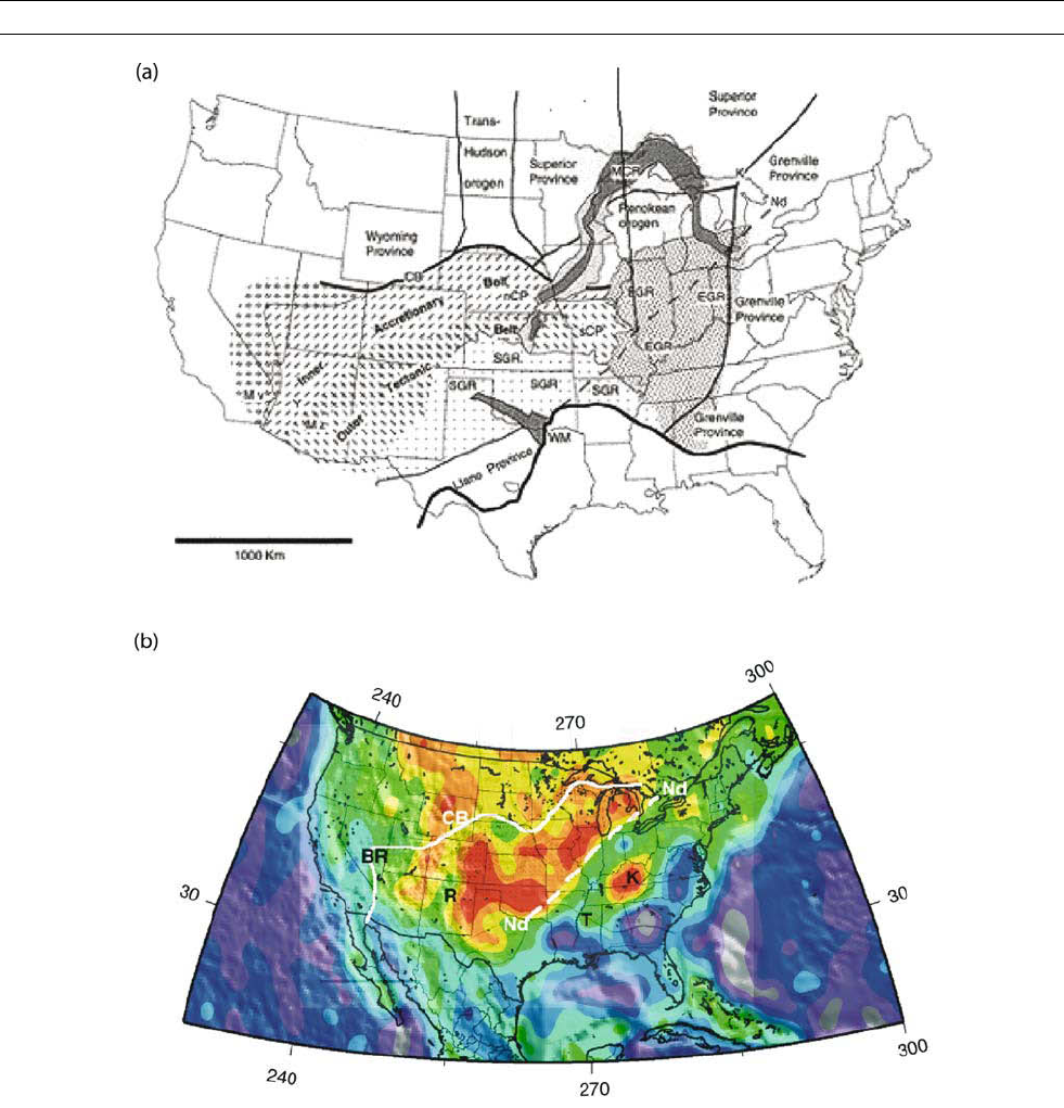
samples throughout the continents. Figure C47a (Plate 6d) shows geo-

logic provinces based on the latest igneous activity in the United States

(Van Schmus et al., 1996). In the western portion (for example, the

western margin of the Inner Accretionary Belt in Figure C47a and

Plate 6d), the geochemical age boundaries well-document the nature

in which the continent accreted during the Middle Proterozoic times

(1.9–1.6 Ga); however, in the eastern part, later igneous activity of the

eastern and southern Granite-Rhyolite provinces (EGR (1470  30 Ma)

and SGR (1370  30 Ma)) obscure the fundamental accretionary

boundaries. It is only through the analyses of Nd isotope data, the crustal

formation age boundary could be defined (shown by a dashed line Nd

in Figure C47a and Plate 6d;VanSchmuset al., 1996) and shown by

a white dashed line in Figure C47b and Plate 6d). The magnetization varia-

tion plotted in Figure C47b (Plate 6d) is the integrated effect of magnetic

CRUSTAL MAGNETIC FIELD 141

property over the thickness of the magnetic layer; it is based on CHAMP

satellite’s MF3 crustal magnetic field model (Maus et al.,2004),which

is much higher resolution data than its predecessors. The depth inte-

grated magnetic property variation is clearly able to delineate the Nd

boundary and reasonably well enclose the Middle Proterozoic province

to the west where it is not affected by later tectonic activity reducing

the thickness of the magnetic layer (e.g., Rio Grande Rift (R) and Basin

and Range Province (BR)). Since the depth integrated magnetic property

map is available for the whole world, it could be used to understand

better the evolution of the less understood parts of Africa, Antarctica, Asia,

Australia, and South America.

In general, the depth integrated magnetic property variation is a

good reflection of large changes in magnetic properties of the bulk

crust in the continents in locations where the crustal thickness does

not vary significantly and also of places where the magnetic crust is

thinner compared to the surrounding regions either because the heat

flow is high (as in the Rio Grande Rift) or because much of the crust

involves nonmagnetic rocks (south of Oklahoma-Alabama transform

(T in Figure C47b/Plate 6d) which was the Precambrian continental

boundary) and sometimes because of the effect of regional remanent

magnetization.

The interpret ation methods

The main purpose of the analysis of the crustal magnetic field is to

gain knowledge of the crustal geology and its geometry, tectonics,

and the evolution of the crust through time. A number of methods

have been developed over the past two centuries that allow geophysi-

cists to work toward this goal. The methods fall into two broad cate-

gories: qualitative and quantitative methods. Qualitative methods use

patterns, magnitude, and wavenumber characteristics of the variation

of the magnetic field to identify, group, and contrast adjacent regions

into geologic domains, subdomains, and cross-cutting features. For

example, referring to Figure C46/Plate 7c, the central region has a sig-

nificantly different magnetic character than the territories on the west

and the east and they can be identified as separate geologic domains

on the basis of magnetic pattern. Magnetic highs associated with

greenstone belts have significantly different signature than the sur-

rounding magnetic highs, reflecting the structural and compositional

variations of the craton. One can also identify, due to their linearity

(and high wavenumber nature), the dikes and faults that cut across

all the geologic domains and the ones that terminate at the edge of

the domains, indicating relative timing of the geologic events. Differ-

ences in wavenumber content usually also imply differences in depths

to magnetic sources—higher wave numbers nearly always arising

from narrow sources reaching closer to the surface. Qualitative corre-

lations among magnetic and other geologic/geophysical information

is also immensely useful in the process of interpretation. Many quali-

tative interpretation tools have their foundation in potential field theory

and mathematical computations of various quantities (e.g., regional/

residual separation, upward/downward continuation and other filtering

techniques), but they are analyzed and interpreted subjectively.

Quantitative methods of analyses can also be subdivided into var-

ious categories, but generally the purpose is to generate a physical

model resembling geology either through iterative matching of mag-

netic anomalies from hypothesized magnetic blocks (called “forward

modeling” when interpreters judge the changes to be made and

“inverse modeling” when matrix inversions and numerical schemes

are formulated to judge the adequacy and nature of the changes)

(Blakely, 1995) or by coming up with particular characteristics of the

Figure C46/Plate 7c A low-altitude, high-resolution aeromagnetic map of a part of the Archean craton in Western Australia

depicting the power of remotely sensed magnetic anomalies in peeling off the sedimentary cover. Pixel size is 25 m which makes it

possible to observe subtle variations in the textures of the buried craton. The aeromagnetic image is courtesy of Fugro Airborne Surveys

Limited. The example is courtesy of Colin Reeves.

142 CRUSTAL MAGNETIC FIELD

nature of the sources (e.g., depths to the top, center or bottom (see

Euler deconvolution)) through analysis of widths, slopes, and ampli-

tudes of isolated anomalies and their derivative fields from different

concentrated geometries (e.g., Analytic Signal method, Euler deconvo-

lution (q.v.) method in Blakely, 1995; Salem and Ravat, 2004),

through the analysis of spectral properties of the field (the Spector

and Grant method, the wavenumber domain centroid method of

Bhattacharyya and Leu in Blakely, 1995; Fedi et al., 1997) through

anomaly attenuation rates and shape factors (see references in Salem

et al., 2005), bounds on physical property contrasts (ideal body theory

of Parker, 1974, 1975 in Blakely, 1995). Unconstrained modeling is

usually not useful in the interpretation of magnetic anomalies because

Figure C47/Plate 6d a, Middle Proterozoic (1.9–1.6 Ga) crustal provinces in the United States: bounded on the north and west by

Mojave Province (Mv), Cheyenne Belt (CB), and continuing up to the Killarney region (k in the northeast) of Ontario. SGR and EGR

are southern Granite-Rhyolite and eastern Granite-Rhyolite provinces. Dashed line (Nd) represents inferred southeastern limit as

defined by Nd isotopic data which bounds the Middle Proterozoic crustal provinces on its southeastern margin and divides SGR

and EGR provinces (from Van Schmus et al., 1996). b, Depth integrated magnetic contrasts over the United States. Orange/reds are

the relative highs in the susceptibility variation and blue/light greens depict relative susceptibility lows. White continuous and

dashed lines (Nd) show the Middle Proterozoic provinces in the United States. Mv from part “a” is excluded from the Middle

Proterozoic region because presently this region is governed by the high heat flow related to the Basin and Range province (BR),

which has decreased the magnetic thickness of the crust and hence it does not appear as a magnetic high. R, Rio Grande Rift; CB,

Cheyenne Belt; K, Kentucky magnetic anomaly; T, Oklahoma-Alabama transform.

CRUSTAL MAGNETIC FIELD 143

of nonuniqueness of potential fields (which theoretically allows infi-

nite number of different configurations to reproduce the same anom-

aly) and the only recourse is to employ constraints derived from

corollary information (e.g., geologic mapping, borehole information,

depths from seismic surveys, etc.) that reduce the ambiguity and

lead to meaningful solutions for the particular geologic situation.

Nonetheless, when all these aspects of interpretation are carefully applied

and limitations assessed, magnetic field provides one of the most valuable

tools for insights into the geology and geophysics of the crust.

Dhananjay Ravat

Bibliography

Blakely, R.J., 1995. Potential Theory in Gravity and Magnetic Appli-

cations. Cambridge: Cambrige University Press.

Keating, P., 1995. A simple technique to identify magnetic anomalies

due to kimberlite pipes. Exploration and Mining Geology, 4:

121–125.

Langel, R.A., Hinze, W.J., 1998. The Magnetic Field of the Earth’s

Lithosphere: The Satellite Perspective. Cambridge: Cambridge

University Press.

Maus, S., Dimri, V.P., 1994. Scaling properties of potential field due to

scaling sources. Geophysical Research Letters, 21: 891–894.

Maus, S., Rother, M., Hemant, K., Lühr, H., Kuvshinov, A., Olsen, N.,

2004. Earth’ s crustal magnetic field determined to spherical harmo-

nic degree 90 from CHAMP satellite measurements. Unpublished

manuscript.

McEnroe, S.A., Brown, L.L., Robinson, P., 2004. Earth analog

for Martian magnetic anomalies: remanence properties of

hemo-ilmenite norites in the Bjerkreim-Sokndal intrusion,

Rogaland, Norway. Journal of Applied Geophysics, 56: 195–212.

Ravat, D., Hildenbrand, T.G., Roest, W., 2003. New way of processing

near-surface magnetic data: The utility of the comprehensive model

of the magnetic field. The Leading Edge, 22: 784– 785.

Sabaka, T.J., Olsen, N., Langel, R.A., 2002. A comprehensive model

of the quiet-time, near-Earth magnetic field: phase 3. Geophysical

Journal International, 151:32–68.

Salem, A., Ravat, D., 2004. A combined analytic signal and Euler

method (AN-EUL) for automatic interpretation of magnetic data.

Geophysics, 68: 1952–1961.

Salem, A., Ravat, D., Smith, R., Ushijima, K., 2005. Interpretation of

magnetic data using an Enhanced Local Wavenumber (ELW)

method. Geophysics, 70:L7–L12.

Van Schmus, W.R, Bickford, M.E., Turek A., 1996. Proterozoic geol-

ogy of the east-central Midcontinent basement. Geological Society

of America Special Paper, 308:7–32.

Cross-references

Aeromagnetic Surveying

Coast Effect of Induced Currents

Core, Electrical Conductivity

Euler Deconvolution

Geomagnetic Secular Variation

Geomagnetic Spectrum, Spatial

IGRF, International Geomagnetic Reference Field

Magnetic Anomalies for Geology and Resources

Magnetic Anomalies, Marine

Magnetization, Natural Remanent (NRM)

Main Field Maps

Mantle, Electrical Conductivity, Mineralogy

Reduction to Pole

Upward and Downward Continuation

144 CRUSTAL MAGNETIC FIELD

AND F-LAYERS

is the rather obscure name for the lowermost mantle adjacent to the

liquid core. The encyclopedia contains several articles on the proper-

ties of D

because of its potential influence on the geodynamo. F is

the name for the boundary layer at the bottom of the outer core, where

liquid core material freezes and differentiates. K.E. Bullen, in 1940–

1942, defined the layers of the Earth on the basis of extensive seismo-

logical studies linked to probable compositional and mineralogical

models. He labelled the layers A to G from the top down, with A

the crust, B the upper mantle, C the transition zone, D the lower

mantle, E the liquid core, F the layer around the inner core, and G

the solid inner core itself (see Earth structure, major divisions).

The F-layer was originally proposed to explain a transition region at

the bottom of the outer core, introduced by H. Jeffreys in 1939, in

which the P-wave velocity decreased with depth. A similar structure

was proposed by Gutenberg (1959). Bullen’s F-layer was 150 km

thick with P-velocity decreasing by about 10% (Bullen and Bolt

(1985), p. 317; Lay and Wallace (1995), p. 305). The evidence for

Jeffrey’s transition zone and the dramatic change in seismic velocity

were removed when seismic arrays made possible the measurement of

slowness (arrival direction): energy thought to be refracted in the F-layer

around the inner core was in fact being scattered from anomalous structure

in the lowermost mantle (Doornbos and Husebye, 1972; Haddon and

Cleary, 1974).

Region D was therefore separated into D

, the lowest few hundred

kilometres of the lower mantle, and D

, the rest of the lower mantle.

Region F was abandoned for lack of seismological evidence, but the

name remained in use in geomagnetism to denote the boundary layer

around the inner core, Braginsky (1963) having already proposed a

theory of energy sources for the geodynamo (q.v.) based on freezing

and differentiating of the liquid close to the inner core. Ironically,

the only parts of Bullen’s original nomenclature in use today is D

not part of the original list, and F, which no longer exists.

The properties of D

are described in the next four articles. It is

thought to be a thermo-chemical boundary layer with large variations

in both temperature and composition that may influence the geody-

namo (see Core-mantle coupling; Electromagnetic; Thermal; and

Topographic). Freezing at the inner core boundary is now thought to

result in a thin mushy zone at the top of the inner core (see Chemical

convection).

David Gubbins

Bibliography

Braginsky, S.I., 1963. Structure of the F layer and reasons for convec-

tion in the Earth’s core. Dokl. Akad. Nauk. SSSR English Transla-

tion, 149: 1311–1314.

Bullen, K.E., and Bolt, B.A., 1985. An Introduction to the Theory of

Seismology. Cambridge: Cambridge University Press.

Doornbos, D.J., and Husebye, E.S., 1972. Array analysis of PKP

phases and their precursors. Physics of the Earth and Planetary

Interiors, 5: 387–399.

Gutenberg, B., 1959. Physics of the Earth’s Interior. New York:

Academic Press.

Haddon, R.A.W., and Cleary, J.R., 1974. Evidence for scattering of

seismic PKP waves near the mantle-core boundary. Physics of

the Earth and Planetary Interiors, 8:211–234.

Lay, T., and Wallace, T.C., 1995. Modern Global Seismology. New York:

Academic Press.

Cross-references

Chemical Convection

Core-Mantle Coupling, Electromagnetic

Core-Mantle Coupling, Thermal

Core-Mantle Coupling, Topographic

Earth Structure, Major Divisions

Energy Sources for the Geodynamo

AS A BOUNDARY LAYER

A boundary layer is a thin region (usually situated near a boundary) in

a fluid or deformable body that has unusual structural properties. In

self-gravitating bodies such as Earth, these regions are characterized

by large gradients of temperature or composition or both. The litho-

sphere is a well-known example of a boundary layer; it is characterized

by both a large gradient of temperature and by long-lived chemical

heterogeneities (including the continents). The D

layer near the base

of Earth’s mantle is believed to have properties complementary to

those of the lithosphere, including a large temperature gradient and

chemical variations. The focus of this article is on the causes and con-

sequences of its thermal structure; its compositional structure is the

subject of a separate entry (see D

, composition).