Greene W.H. Econometric Analysis

Подождите немного. Документ загружается.

CHAPTER 20

✦

Serial Correlation

929

is statistically signiﬁcant in this auxiliary, second-step regression. Another indicator is

provided by the FGLS residuals, themselves. After computing the FGLS regression,

the estimated residuals,

ˆε = y

− x



will still be autocorrelated. In our results using the Prais–Winsten estimates, the auto-

correlation of the FGLS residuals is 0.957. The associated Durbin–Watson statistic is

0.0867. This is to be expected. However, if the model is correct, then the transformed

residuals

ˆu

= ˆε

− ˆρ ˆε

t−1

should be at least close to nonautocorrelated. But, for our data, the autocorrelation of

these adjusted residuals is only 0.292 with a Durbin–Watson statistic of 1.416. The value

of d

for one regressor (u

t−1

) and 50 observations is 1.50. It appears on this basis that,

in fact, the AR(1) model has largely completed the speciﬁcation.

20.9.3 ESTIMATION WITH A LAGGED DEPENDENT VARIABLE

In Section 20.5.1, we considered the problem of estimation by least squares when the

model contains both autocorrelation and lagged dependent variable(s). Because the

OLS estimator is inconsistent, the residuals on which an estimator of ρ would be based

are likewise inconsistent. Therefore, ˆρ will be inconsistent as well. The consequence

is that the FGLS estimators described earlier are not usable in this case. There is,

however, an alternative way to proceed, based on the method of instrumental variables.

The method of instrumental variables was introduced in Section 8.3.2. To review, the

general problem is that in the regression model, if

plim(1/T )X



ε = 0,

then the least squares estimator is not consistent. A consistent estimator is

= (Z



−1



y),

where Z is a set of K variables chosen such that plim(1/T)Z



ε = 0 but plim(1/T)Z



X =

0. For the purpose of consistency only, any such set of instrumental variables will sufﬁce.

The relevance of that here is that the obstacle to consistent FGLS is, at least for the

present, is the lack of a consistent estimator of ρ. By using the technique of instrumental

variables, we may estimate β consistently, then estimate ρ and proceed.

Hatanaka (1974, 1976) has devised an efﬁcient two-step estimator based on this prin-

ciple. To put the estimator in the current context, we consider estimation of the model

= x



β + γ y

t−1

+ ε

= ρε

t−1

+ u

To get to the second step of FGLS, we require a consistent estimator of the slope pa-

rameters. These estimates can be obtained using an IV estimator, where the column

of Z corresponding to y

t−1

is the only one that need be different from that of X.An

appropriate instrument can be obtained by using the ﬁtted values in the regression of

on x

and x

t−1

. The residuals from the IV regression are then used to construct

ˆρ =



t=3

ˆε

t−1



t=3

ˆε

, (20-33)

930

PART V

✦

Time Series and Macroeconometrics

where

ˆε

= y

− b



− c

t−1

FGLS estimates may now be computed by regressing y

∗

= y

− ˆρ y

t−1

∗

= x

− ˆρx

t−1

∗

t−1

= y

t−1

− ˆρ y

t−2

ˆε

t−1

= y

t−1

− b



t−1

− c

t−2

Let d be the coefﬁcient on ˆε

t−1

in this regression. The efﬁcient estimator of ρ is

ˆρ = ˆρ + d.

Appropriate asymptotic standard errors for the estimators, including

ˆρ, are obtained

from the s



∗

]

−1

computed at the second step. Hatanaka shows that these estimators

are asymptotically equivalent to maximum likelihood estimators.

20.10 AUTOREGRESSIVE CONDITIONAL

HETEROSCEDASTICITY

Heteroscedasticity is often associated with cross-sectional data, whereas time series are

usually studied in the context of homoscedastic processes. In analyses of macroeconomic

data, Engle (1982, 1983) and Cragg (1982) found evidence that for some kinds of data,

the disturbance variances in time-series models were less stable than usually assumed.

Engle’s results suggested that in models of inﬂation, large and small forecast errors

appeared to occur in clusters, suggesting a form of heteroscedasticity in which the

variance of the forecast error depends on the size of the previous disturbance. He

suggested the autoregressive, conditionally heteroscedastic, or ARCH, model as an

alternative to the usual time-series process. More recent studies of ﬁnancial markets

suggest that the phenomenon is quite common. The ARCH model has proven to be

useful in studying the volatility of inﬂation [Coulson and Robins (1985)], the term

structure of interest rates [Engle, Hendry, and Trumble (1985)], the volatility of stock

market returns [Engle, Lilien, and Robins (1987)], and the behavior of foreign exchange

markets [Domowitz and Hakkio (1985) and Bollerslev and Ghysels (1996)], to name

but a few. This section will describe speciﬁcation, estimation, and testing, in the basic

formulations of the ARCH model and some extensions.

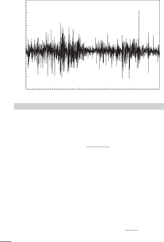
Example 20.5 Stochastic Volatility

Figure 20.5 shows Bollerslev and Ghysel’s 1974 data on the daily percentage nominal return

for the Deutschmark/Pound exchange rate. (These data are given in Appendix Table F20.1.)

The variation in the series appears to be ﬂuctuating, with several clusters of large and small

movements.

See Section 14.9.2.b.

Engle and Rothschild (1992) give a survey of this literature which describes many extensions. Mills (1993)

also presents several applications. See, as well, Bollerslev (1986) and Li, Ling, and McAleer (2001). See

McCullough and Renfro (1999) for discussion of estimation of this model.

CHAPTER 20

✦

Serial Correlation

931

0 395 790 1185

Observation Number

1580 1975

3

2

1

FIGURE 20.5

Nominal Exchange Rate Returns.

20.10.1 THE ARCH(1) MODEL

The simplest form of this model is the ARCH(1) model,

= x



β + ε

= u

+ α

t−1

(20-34)

where u

is distributed as standard normal.

It follows that E [ε

,ε

t−1

] = 0, so that

E [ε

] = 0 and E [y

] = x



β. Therefore, this model is a classical regression model.

But

Var[ε

|ε

t−1

] = E



t−1



= E





+ α

t−1



= α

+ α

t−1

so ε

is conditionally heteroscedastic, not with respect to x

as we considered in Chapter 9,

but with respect to ε

t−1

. The unconditional variance of ε

Var[ε

] = Va r



E [ε

|ε

t−1

]



+ E



Var[ε

|ε

t−1

]



= α

+ α



t−1



= α

+ α

Var[ε

t−1

If the process generating the disturbances is weakly (covariance) stationary (see Deﬁ-

nition 19.2),

then the unconditional variance is not changing over time so

Var[ε

] = Var[ε

t−1

] = α

+ α

Var[ε

t−1

] =

1 − α

The assumption that u

has unit variance is not a restriction. The scaling implied by any other variance

would be absorbed by the other parameters.

This discussion will draw on the results and terminology of time-series analysis in Section 20.3. The reader

may wish to peruse this material at this point.

932

PART V

✦

Time Series and Macroeconometrics

For this ratio to be ﬁnite and positive, |α

| must be less than 1. Then, unconditionally,

is distributed with mean zero and variance σ

= α

/(1 − α

). Therefore, the model

obeys the classical assumptions, and ordinary least squares is the most efﬁcient linear

unbiased estimator of β.

But there is a more efﬁcient nonlinear estimator. The log-likelihood function for

this model is given by Engle (1982). Conditioned on starting values y

and x

(and ε

the conditional log-likelihood for observations t = 1,...,T is the one we examined in

Section 14.9.2.a for the general heteroscedastic regression model [see (14-52)],

ln L =−

ln(2π) −



t=1



+ α

t−1



−



t=1

+ α

t−1

,ε

= y

− β



(20-35)

Maximization of log L can be done with the conventional methods, as discussed in

Appendix E.

20.10.2 ARCH(

), ARCH-IN-MEAN, AND GENERALIZED

ARCH MODELS

The natural extension of the ARCH(1) model presented before is a more general model

with longer lags. The ARCH(q) process,

= α

+ α

t−1

+ α

t−2

+···+α

t−q

is a qth order moving average [MA(q)] process. [Once again, see Engle (1982).] This

section will generalize the ARCH(q) model, as suggested by Bollerslev (1986), in the

direction of the autoregressive-moving average (ARMA) models of Section 22.2.1. The

discussion will parallel his development, although many details are omitted for brevity.

The reader is referred to that paper for background and for some of the less critical

details.

Among the many variants of the capital asset pricing model (CAPM) is an intertem-

poral formulation by Merton (1980) that suggests an approximate linear relationship

between the return and variance of the market portfolio. One of the possible ﬂaws

in this model is its assumption of a constant variance of the market portfolio. In this

connection, then, the ARCH-in-Mean, or ARCH-M, model suggested by Engle, Lilien,

and Robins (1987) is a natural extension. The model states that

= β



+ δσ

+ ε

Var[ε

|

] = ARCH(q).

Among the interesting implications of this modiﬁcation of the standard model is that

under certain assumptions, δ is the coefﬁcient of relative risk aversion. The ARCH-M

model has been applied in a wide variety of studies of volatility in asset returns, including

Engle (1982) and Judge et al. (1985, pp. 441– 444) suggest a four-step procedure based on the method

of scoring that resembles the two-step method we used for the multiplicative heteroscedasticity model in

Section 8.8.1. However, the full MLE is now incorporated in most modern software, so the simple regres-

sion based methods, which are difﬁcult to generalize, are less attractive in the current literature. But, see

McCullough and Renfro (1999) and Fiorentini, Calzolari, and Panattoni (1996) for commentary and some

cautions related to maximum likelihood estimation.

CHAPTER 20

✦

Serial Correlation

933

the daily Standard and Poor’s Index [French, Schwert, and Stambaugh (1987)] and

weekly New York Stock Exchange returns [Chou (1988)]. A lengthy list of applications

is given in Bollerslev, Chou, and Kroner (1992).

The ARCH-M model has several noteworthy statistical characteristics. Unlike the

standard regression model, misspeciﬁcation of the variance function does affect the

consistency of estimators of the parameters of the mean. [See Pagan and Ullah (1988)

for formal analysis of this point.] Recall that in the classical regression setting, weighted

least squares is consistent even if the weights are misspeciﬁed as long as the weights are

uncorrelated with the disturbances. That is not true here. If the ARCH part of the model

is misspeciﬁed, then conventional estimators of β and δ will not be consistent. Bollerslev,

Chou, and Kroner (1992) list a large number of studies that called into question the

speciﬁcation of the ARCH-M model, and they subsequently obtained quite different

results after respecifying the model. A closely related practical problem is that the

mean and variance parameters in this model are no longer uncorrelated. In analysis

up to this point, we made quite proﬁtable use of the block diagonality of the Hessian

of the log-likelihood function for the model of heteroscedasticity. But the Hessian for

the ARCH-M model is not block diagonal. In practical terms, the estimation problem

cannot be segmented as we have done previously with the heteroscedastic regression

model. All the parameters must be estimated simultaneously.

The model of generalized autoregressive conditional heteroscedasticity (GARCH)

is deﬁned as follows.

The underlying regression is the usual one in (20-34). Conditioned

on an information set at time t, denoted 

, the distribution of the disturbance is assumed

to be

|

∼ N



0,σ



where the conditional variance is

= α

+ δ

t−1

+ δ

t−2

+···+δ

t−p

+ α

t−1

+ α

t−2

+···+α

t−q

. (20-36)

Deﬁne



1,σ

t−1

,σ

t−2

,...,σ

t−p

,ε

t−1

,ε

t−2

,...,ε

t−q





and

γ = [α

,δ

,...,δ

,α

,...,α

]



= [α

, δ



, α



]



Then

= γ



Notice that the conditional variance is deﬁned by an autoregressive-moving average

[ARMA ( p, q)] process in the innovations ε

. The difference here is that the mean of

the random variable of interest y

is described completely by a heteroscedastic, but

otherwise ordinary, regression model. The conditional variance, however, evolves over

time in what might be a very complicated manner, depending on the parameter values

and on p and q. The model in (20-36) is a GARCH(p, q) model, where p refers, as

As have most areas in time-series econometrics, the line of literature on GARCH models has progressed

rapidly in recent years and will surely continue to do so. We have presented Bollerslev’s model in some detail,

despite many recent extensions, not only to introduce the topic as a bridge to the literature, but also because it

provides a convenient and interesting setting in which to discuss several related topics such as double-length

regression and pseudo–maximum likelihood estimation.

934

PART V

✦

Time Series and Macroeconometrics

before, to the order of the autoregressive part.

As Bollerslev (1986) demonstrates with

an example, the virtue of this approach is that a GARCH model with a small number

of terms appears to perform as well as or better than an ARCH model with many.

The stationarity conditions are important in this context to ensure that the moments

of the normal distribution are ﬁnite. The reason is that higher moments of the normal

distribution are ﬁnite powers of the variance. A normal distribution with variance σ

has fourth moment 3σ

, sixth moment 15σ

, and so on. [The precise relationship of

the even moments of the normal distribution to the variance is μ

=(σ

)

(2k)!/(k!2

).]

Simply ensuring that σ

is stable does not ensure that higher powers are as well.

Bollerslev presents a useful ﬁgure that shows the conditions needed to ensure stability

for moments up to order 12 for a GARCH(1, 1) model and gives some additional

discussion. For example, for a GARCH(1, 1) process, for the fourth moment to exist,

3α

+ 2α

+ δ

must be less than 1.

It is convenient to write (20-36) in terms of polynomials in the lag operator;

= α

+ D(L)σ

+ A(L)ε

The stationarity condition for such an equation is that the roots of the characteristic

equation, 1 − D(z) = 0, must lie outside the unit circle. For the present, we will as-

sume that this case is true for the model we are considering and that A(1) + D(1)<1.

[This assumption is stronger than that needed to ensure stationarity in a higher-order

autoregressive model, which would depend only on D(L).] The implication is that the

GARCH process is covariance stationary with E [ε

] = 0 (unconditionally), Var[ε

] =

/[1 − A(1) − D(1)], and Cov[ε

,ε

] = 0 for all t = s. Thus, unconditionally the model

is the classical regression model that we examined in Chapters 2–6.

The usefulness of the GARCH speciﬁcation is that it allows the variance to evolve

over time in a way that is much more general than the simple speciﬁcation of the ARCH

model. For the example discussed in his paper, Bollerslev reports that although Engle

and Kraft’s (1983) ARCH(8) model for the rate of inﬂation in the GNP deﬂator appears

to remove all ARCH effects, a closer look reveals GARCH effects at several lags. By

ﬁtting a GARCH(1, 1) model to the same data, Bollerslev ﬁnds that the ARCH effects

out to the same eight-period lag as ﬁt by Engle and Kraft and his observed GARCH

effects are all satisfactorily accounted for.

20.10.3 MAXIMUM LIKELIHOOD ESTIMATION

OF THE GARCH MODEL

Bollerslev describes a method of estimation based on the BHHH algorithm. As he

shows, the method is relatively simple, although with the line search and ﬁrst derivative

method that he suggests, it probably involves more computation and more iterations

than necessary. Following the suggestions of Harvey (1976), it turns out that there is a

simpler way to estimate the GARCH model that is also very illuminating. This model is

actually very similar to the more conventional model of multiplicative heteroscedasticity

that we examined in Section 14.9.2.a.

We have changed Bollerslev’s notation slightly so as not to conﬂict with our previous presentation. He used

β instead of our δ in (20-36) and b instead of our β in (20-34).

The conditions cannot be imposed a priori. In fact, there is no nonzero set of parameters that guarantees

stability of all moments, even though the normal distribution has ﬁnite moments of all orders. As such, the

normality assumption must be viewed as an approximation.

CHAPTER 20

✦

Serial Correlation

935

For normally distributed disturbances, the log-likelihood for a sample of T obser-

vations is

ln L =



t=1

−



ln(2π) + ln σ





t=1

ln f

(θ) =



t=1

(θ),

where ε

= y

−x



β and θ = (β



, α



, δ



)



= (β



, γ



)



. Derivatives of ln L are obtained

by summation. Let l

denote ln f

(θ). The ﬁrst derivatives with respect to the variance

parameters are

∂l

∂γ

=−



−







∂σ

∂γ





∂σ

∂γ



− 1







= b

(20-37)

Note that E [v

] = 0. Suppose, for now, that there are no regression parameters.

Newton’s method for estimating the variance parameters would be

ˆγ

i+1

= ˆγ

− H

−1

g, (20-38)

where H indicates the Hessian and g is the ﬁrst derivatives vector. Following Harvey’s

suggestion (see Section 14.9.2.a), we will use the method of scoring instead. To do this,

we make use of E [v

] =0 and E [ε

/σ

] =1. After taking expectations in (20-37), the it-

eration reduces to a linear regression of v

∗

=(1/

√

2)v

on regressors w

∗

=(1/

√

2)g

/σ

That is,

ˆγ

i+1

= ˆγ

+ [W



∗

]

−1



∗

= ˆγ

+ [W



∗

]

−1



∂ ln L

∂γ



, (20-39)

where row t of W

∗

is w



∗

. The iteration has converged when the slope vector is zero,

which happens when the ﬁrst derivative vector is zero. When the iterations are complete,

the estimated asymptotic covariance matrix is simply

Est. Asy. Var[ ˆγ ] = [



∗

]

−1

based on the estimated parameters.

The usefulness of the result just given is that E [∂

ln L/∂γ ∂β



] is, in fact, zero. Be-

cause the expected Hessian is block diagonal, applying the method of scoring to the full

parameter vector can proceed in two parts, exactly as it did in Section 14.9.2.a for the

multiplicative heteroscedasticity model. That is, the updates for the mean and variance

parameter vectors can be computed separately. Consider then the slope parameters, β.

The same type of modiﬁed scoring method as used earlier produces the iteration

i+1





t=1













−1





t=1











t=1













−1



∂ ln L

∂β



(20-40)

+ h

There are three minor errors in Bollerslev’s derivation that we note here to avoid the apparent inconsisten-

cies. In his (22),

should be

−1

. In (23), −2h

−2

should be −h

−2

. In (28), h ∂h/∂ω should, in each case,

be (1/ h)∂h/∂ω. [In his (8), α

should be α

+ α

, but this has no implications for our derivation.]

936

PART V

✦

Time Series and Macroeconometrics

which has been referred to as a double-length regression. [See Orme (1990) and David-

son and MacKinnon (1993, Chapter 14).] The update vector h

is the vector of slopes

in an augmented or double-length generalized regression,

= [C





−1





−1

a], (20-41)

where C isa2T × K matrix whose ﬁrst T rows are the X from the original regression

model and whose next T rows are (1/

√

2)d



/σ

, t = 1,...,T; a isa2T ×1 vector whose

ﬁrst T elements are ε

and whose next T elements are (1/

√

2)v

/σ

, t = 1,...,T; and

 is a diagonal matrix with 1/σ

in positions 1,...,T and ones below observation T.

At convergence, [C





−1

provides the asymptotic covariance matrix for the MLE.

The resemblance to the familiar result for the generalized regression model is striking,

but note that this result is based on the double-length regression.

The iteration is done simply by computing the update vectors to the current pa-

rameters as deﬁned earlier.

An important consideration is that to apply the scoring

method, the estimates of β and γ are updated simultaneously. That is, one does not use

the updated estimate of γ in (20-39) to update the weights for the GLS regression to

compute the new β in (20-40). The same estimates (the results of the prior iteration) are

used on the right-hand sides of both (20-39) and (20-40). The remaining problem is to

obtain starting values for the iterations. One obvious choice is b, the OLS estimator, for

β, e



e/T =s

for α

, and zero for all the remaining parameters. The OLS slope vector

will be consistent under all speciﬁcations. A useful alternative in this context would be

to start α at the vector of slopes in the least squares regression of e

, the squared OLS

residual, on a constant and q lagged values.

As discussed later, an LM test for the

presence of GARCH effects is then a by-product of the ﬁrst iteration. In principle, the

updated result of the ﬁrst iteration is an efﬁcient two-step estimator of all the parame-

ters. But having gone to the full effort to set up the iterations, nothing is gained by not

iterating to convergence. One virtue of allowing the procedure to iterate to convergence

is that the resulting log-likelihood function can be used in likelihood ratio tests.

20.10.4 TESTING FOR GARCH EFFECTS

The preceding development appears fairly complicated. In fact, it is not, because at each

step, nothing more than a linear least squares regression is required. The intricate part

of the computation is setting up the derivatives. On the other hand, it does take a fair

amount of programming to get this far.

As Bollerslev suggests, it might be useful to

test for GARCH effects ﬁrst.

The simplest approach is to examine the squares of the least squares residuals.

The autocorrelations (correlations with lagged values) of the squares of the residuals

provide evidence about ARCH effects. An LM test of ARCH(q) against the hypothesis

of no ARCH effects [ARCH(0), the classical model] can be carried out by computing

=TR

in the regression of e

on a constant and q lagged values. Under the null

See Fiorentini et al. (1996) on computation of derivatives in GARCH models.

A test for the presence of q ARCH effects against none can be carried out by carrying TR

from this

regression into a table of critical values for the chi-squared distribution. But in the presence of GARCH

effects, this procedure loses its validity.

Because this procedure is available as a preprogrammed procedure in many computer programs, including

TSP, E-Views, Stata, RATS, LIMDEP, and Shazam, this warning might itself be overstated.

CHAPTER 20

✦

Serial Correlation

937

TABLE 20.3

Maximum Likelihood Estimates of a GARCH(1, 1) Model

μα

δα

/(1 − α

− δ)

Estimate −0.006190 0.01076 0.1531 0.8060 0.2631

Std. Error 0.00873 0.00312 0.0273 0.0302 0.594

t ratio −0.709 3.445 5.605 26.731 0.443

ln L =−1106.61, ln L

OLS

=−1311.09, ¯y =−0.01642, s

= 0.221128

hypothesis of no ARCH effects, the statistic has a limiting chi-squared distribution with

q degrees of freedom. Values larger than the critical table value give evidence of the

presence of ARCH (or GARCH) effects.

Bollerslev suggests a Lagrange multiplier statistic that is, in fact, surprisingly simple

to compute. The LM test for GARCH( p, 0) against GARCH( p, q) can be carried out

by referring T times the R

in the linear regression deﬁned in (20-42) to the chi-squared

critical value with q degrees of freedom. There is, unfortunately, an indeterminacy in

this test procedure. The test for ARCH(q) against GARCH(p, q) is exactly the same

as that for ARCH( p) against ARCH( p + q). For carrying out the test, one can use as

starting values a set of estimates that includes δ = 0 and any consistent estimators for

β and α. Then TR

for the regression at the initial iteration provides the test statistic.

A number of recent papers have questioned the use of test statistics based solely

on normality. Wooldridge (1991) is a useful summary with several examples.

Example 20.6 GARCH Model for Exchange Rate Volatility

Bollerslev and Ghysels analyzed the exchange rate data in Example 20.7 using a GARCH(1, 1)

model,

= μ + ε

E[ε

|ε

t−1

] = 0,

Var[ε

|ε

t−1

] = σ

= α

+ α

t−1

+ δσ

t−1

The least squares residuals for this model are simply e

= y

− ¯y. Regression of the squares

of these residuals on a constant and 10 lagged squared values using observations 11–1974

produces an R

= 0.09795. With T = 1964, the chi-squared statistic is 192.37, which is larger

than the critical value from the table of 18.31. We conclude that there is evidence of GARCH

effects in these residuals. The maximum likelihood estimates of the GARCH model are given

in Table 20.3. Note the resemblance between the OLS unconditional variance (0.221128) and

the estimated equilibrium variance from the GARCH model, 0.2631.

20.10.5 PSEUDO–MAXIMUM LIKELIHOOD ESTIMATION

We now consider an implication of nonnormality of the disturbances. Suppose that the

assumption of normality is weakened to only

E [ε

|

] = 0, E







= 1, E







= κ<∞,

Bollerslev argues that in view of the complexity of the computations involved in estimating the GARCH

model, it is useful to have a test for GARCH effects. This case is one (as are many other maximum likelihood

problems) in which the apparatus for carrying out the test is the same as that for estimating the model. Having

computed the LM statistic for GARCH effects, one can proceed to estimate the model just by allowing the

program to iterate to convergence. There is no additional cost beyond waiting for the answer.

938

PART V

✦

Time Series and Macroeconometrics

where σ

is as deﬁned earlier. Now the normal log-likelihood function is inappropriate.

In this case, the nonlinear (ordinary or weighted) least squares estimator would have the

properties discussed in Chapter 7. It would be more difﬁcult to compute than the MLE

discussed earlier, however. It has been shown [see White (1982a) and Weiss (1982)]

that the pseudo-MLE obtained by maximizing the same log-likelihood as if it were

correct produces a consistent estimator despite the misspeciﬁcation.

The asymptotic

covariance matrices for the parameter estimators must be adjusted, however.

The general result for cases such as this one [see Gourieroux, Monfort, and Trognon

(1984)] is that the appropriate asymptotic covariance matrix for the pseudo-MLE of a

parameter vector θ would be

Asy. Var[

θ] = H

−1

, (20-42)

where

H =−E



∂

ln L

∂θ ∂θ





and

F = E



∂ ln L

∂θ



∂ ln L

∂θ





(i.e., the BHHH estimator), and ln L is the used but inappropriate log-likelihood func-

tion. For current purposes, H and F are still block diagonal, so we can treat the mean and

variance parameters separately. In addition, E [v

] is still zero, so the second derivative

terms in both blocks are quite simple. (The parts involving ∂

/∂γ ∂γ



and ∂

/∂β ∂β



fall out of the expectation.) Taking expectations and inserting the parts produces the

corrected asymptotic covariance matrix for the variance parameters:

Asy. Var[ ˆγ

PMLE

] = [W



∗

]

−1



B[W



∗

]

−1

where the rows of W

∗

are deﬁned in (20-39) and those of B are in (20-37). For the slope

parameters, the adjusted asymptotic covariance matrix would be

Asy. Var[

PMLE

] = [C





−1





t=1









−1

where the outer matrix is deﬁned in (20-41) and, from the ﬁrst derivatives given in

(20-37) and (20-40),





These data have become a standard data set for the evaluation of software for estimating GARCH models.

The values given are the benchmark estimates. Standard errors differ substantially from one method to the

next. Those given are the Bollerslev and Wooldridge (1992) results. See McCullough and Renfro (1999).

White (1982a) gives some additional requirements for the true underlying density of ε

. Gourieroux,

Monfort, and Trognon (1984) also consider the issue. Under the assumptions given, the expectations of

the matrices in (20-36) and (20-41) remain the same as under normality. The consistency and asymptotic

normality of the pseudo-MLE can be argued under the logic of GMM estimators.

McCullough and Renfro (1999) examined several approaches to computing an appropriate asymptotic

covariance matrix for the GARCH model, including the conventional Hessian and BHHH estimators and

three sandwich style estimators, including the one suggested earlier and two based on the method of scoring

suggested by Bollerslev and Wooldridge (1992). None stand out as obviously better, but the Bollerslev and

QMLE estimator based on an actual Hessian appears to perform well in Monte Carlo studies.