Greene W.H. Econometric Analysis
Подождите немного. Документ загружается.


CHAPTER 20
✦
Serial Correlation
919
and assume |β|< 1, |ρ|< 1. In this model, the regressor and the disturbance are
correlated. There are various ways to approach the analysis. One useful way is to rear-
range (20-12) by subtracting ρy
t−1
from y
t
. Then,
y
t
= (β + ρ)y
t−1
− βρy
t−2
+ u
t
, (20-13)
which is a classical regression with stochastic regressors. Because u
t
is an innovation in
period t, it is uncorrelated with both regressors, and least squares regression of y
t
on
(y
t−1
, y
t−2
) estimates ρ
1
=(β +ρ)and ρ
2
=−βρ. What is estimated by regression of y
t
on
y
t−1
alone? Let γ
k
= Cov[y
t
, y
t−k
] = Cov[y
t
, y
t+k
]. By stationarity, Var[y
t
] = Var[y
t−1
],
and Cov[y
t
, y
t−1
] = Cov[y
t−1
, y
t−2
], and so on. These and (20-13) imply the following
relationships:
γ
0
= ρ
1
γ
1
+ ρ
2
γ
2
+ σ
2
u
,
γ
1
= ρ
1
γ
0
+ ρ
2
γ
1
,
γ
2
= ρ
1
γ
1
+ ρ
2
γ
0
.
(20-14)
(These are the Yule–Walker equations for this model.) The slope in the simple regression
estimates γ
1
/γ
0
, which can be found in the solutions to these three equations. (An
alternative approach is to use the left-out variable formula, which is a useful way to
interpret this estimator.) In this case, we see that the slope in the short regression is an
estimator of (β + ρ) − βρ(γ
1
/γ
0
). In either case, solving the three equations in (20-14)
for γ
0
,γ
1
, and γ
2
in terms of ρ
1
,ρ
2
, and σ
2
u
produces
plim b =
β + ρ
1 + βρ
. (20-15)
This result is between β (when ρ =0) and 1 (when both β and ρ =1). Therefore, least
squares is inconsistent unless ρ equals zero. The more general case that includes re-
gressors, x
t
, involves more complicated algebra but gives essentially the same result.
This is a general result; When the equation contains a lagged dependent variable in
the presence of autocorrelation, OLS and GLS are inconsistent. The problem can be
viewed as one of an omitted variable.
20.5.2 ESTIMATING THE VARIANCE OF THE LEAST
SQUARES ESTIMATOR
As usual, s
2
(X
X)
−1
is an inappropriate estimator of σ
2
(X
X)
−1
(X
X)(X
X)
−1
, both
because s
2
is a biased estimator of σ
2
and because the matrix is incorrect. Generalities
are scarce, but in general, for economic time series that are positively related to their
past values, the standard errors conventionally estimated by least squares are likely to
be too small. For slowly changing, trending aggregates such as output and consumption,
this is probably the norm. For highly variable data such as inflation, exchange rates,
and market returns, the situation is less clear. Nonetheless, as a general proposition,
one would normally not want to rely on s
2
(X
X)
−1
as an estimator of the asymptotic
covariance matrix of the least squares estimator.
In view of this situation, if one is going to use least squares, then it is desirable to
have an appropriate estimator of the covariance matrix of the least squares estimator.
There are two approaches. If the form of the autocorrelation is known, then one can
estimate the parameters of directly and compute a consistent estimator. Of course,

920
PART V
✦
Time Series and Macroeconometrics
if so, then it would be more sensible to use feasible generalized least squares instead
and not waste the sample information on an inefficient estimator. The second approach
parallels the use of the White estimator for heteroscedasticity.
The extension of White’s result to the more general case of autocorrelation is much
more difficult than in the heteroscedasticity case. The natural counterpart for estimating
Q
∗
=
1
n
n
i=1
n
j=1
σ
ij
x
i
x
j
(20-16)
in Section 9.2.3 would be
ˆ
Q
∗
=
1
T
T
t=1
T
s=1
e
t
e
s
x
t
x
s
.
But there are two problems with this estimator, one theoretical, which applies to Q
∗
as
well, and one practical, which is specific to the latter.
Unlike the heteroscedasticity case, the matrix in (20-16) is 1/T times a sum of
T
2
terms, so it is difficult to conclude yet that it will converge to anything at all. This
application is most likely to arise in a time-series setting. To obtain convergence, it is
necessary to assume that the terms involving unequal subscripts in (20-16) diminish in
importance as T grows. A sufficient condition is that terms with subscript pairs |t − s|
grow smaller as the distance between them grows larger. In practical terms, observation
pairs are progressively less correlated as their separation in time grows. Intuitively, if
one can think of weights with the diagonal elements getting a weight of 1.0, then in the
sum, the weights in the sum grow smaller as we move away from the diagonal. If we
think of the sum of the weights rather than just the number of terms, then this sum falls
off sufficiently rapidly that as n grows large, the sum is of order T rather than T
2
. Thus,
we achieve convergence of Q
∗
by assuming that the rows of X are well behaved and
that the correlations diminish with increasing separation in time. (See Section 9.2.2 for
a more formal statement of this condition.)
The practical problem is that
ˆ
Q
∗
need not be positive definite. Newey and West
(1987a) have devised an estimator that overcomes this difficulty:
ˆ
Q
∗
= S
0
+
1
T
L
l=1
T
t=l+1
w
l
e
t
e
t−l
(x
t
x
t−l
+ x
t−l
x
t
),
w
l
= 1 −
l
(L + 1)
.
(20-17)
[See (9-27).] The Newey–West autocorrelation consistent covariance estimator is sur-
prisingly simple and relatively easy to implement.
10
There is a final problem to be solved.
It must be determined in advance how large L is to be. In general, there is little the-
oretical guidance. Current practice specifies L ≈ T
1/4
. Unfortunately, the result is not
quite as crisp as that for the heteroscedasticity consistent estimator.
We have the result that b and b
IV
are asymptotically normally distributed, and
we have an appropriate estimator for the asymptotic covariance matrix. We have not
10
Both estimators are now standard features in modern econometrics computer programs. Further results on
different weighting schemes may be found in Hayashi (2000, pp. 406–410).

CHAPTER 20
✦
Serial Correlation
921
TABLE 20.1
Robust Covariance Estimation
Variable OLS Estimate OLS SE Corrected SE
Constant −1.6331 0.2286 0.3335
ln Output 0.2871 0.04738 0.07806
ln CPI 0.9718 0.03377 0.06585
R
2
=0.98952, d =0.02477, r =0.98762.
specified the distribution of the disturbances, however. Thus, for inference purposes,
the F statistic is approximate at best. Moreover, for more involved hypotheses, the
likelihood ratio and Lagrange multiplier tests are unavailable. That leaves the Wald
statistic, including asymptotic “t ratios,” as the main tool for statistical inference. We
will examine a number of applications in the chapters to follow.
The White and Newey–West estimators are standard in the econometrics literature.
We will encounter them at many points in the discussion to follow.
Example 20.4 Autocorrelation Consistent Covariance Estimation
For the model shown in Example 20.1, the regression results with the uncorrected standard
errors and the Newey–West autocorrelation robust covariance matrix for lags of five quarters
are shown in Table 20.1. The effect of the very high degree of autocorrelation is evident.
20.6 GMM ESTIMATION
The GMM estimator in the regression model with autocorrelated disturbances is pro-
duced by the empirical moment equations
1
T
T
t=1
x
t
y
t
− x
t
ˆ
β
GMM
=
1
T
X
ˆε
ˆ
β
GMM
=
¯
m
ˆ
β
GMM
= 0. (20-18)
The estimator is obtained by minimizing
q =
¯
m
ˆ
β
GMM
W
¯
m
ˆ
β
GMM
where W is a positive definite weighting matrix. The optimal weighting matrix would be
W =
Asy. Var[
√
T
¯
m(β)]
−1
,
which is the inverse of
Asy. Var[
√
T
¯
m(β)] = Asy. Var
1
√
T
n
i=1
x
i
ε
i
= plim
n→∞
1
T
T
t=1
T
s=1
σ
2
ρ
ts
x
t
x
s
= σ
2
Q
∗
.
The optimal weighting matrix would be [σ
2
Q
∗
]
−1
. As in the heteroscedasticity case, this
minimization problem is an exactly identified case, so, the weighting matrix is actually
irrelevant to the solution. The GMM estimator for the regression model with autocor-
related disturbances is ordinary least squares. We can use the results in Section 20.5.2
to construct the asymptotic covariance matrix. We will require the assumptions in Sec-
tion 20.4 to obtain convergence of the moments and asymptotic normality. We will wish
to extend this simple result in one instance. In the common case in which x
t
contains

922
PART V
✦
Time Series and Macroeconometrics
lagged values of y
t
, we will want to use an instrumental variable estimator. We will
return to that estimation problem in Section 20.9.3.
20.7 TESTING FOR AUTOCORRELATION
The available tests for autocorrelation are based on the principle that if the true distur-
bances are autocorrelated, then this fact can be detected through the autocorrelations of
the least squares residuals. The simplest indicator is the slope in the artificial regression
e
t
= re
t−1
+ v
t
,
e
t
= y
t
− x
t
b,
r =
T
t=2
e
t
e
t−1
%
T−1
t=1
e
2
t
.
(20-19)
If there is autocorrelation, then the slope in this regression will be an estimator of
ρ = Corr[ε
t
,ε
t−1
]. The complication in the analysis lies in determining a formal means
of evaluating when the estimator is “large,” that is, on what statistical basis to reject
the null hypothesis that ρ equals zero. As a first approximation, treating (20-19) as a
classical linear model and using a t or F (squared t) test to test the hypothesis is a
valid way to proceed based on the Lagrange multiplier principle. We used this device
in Example 20.3. The tests we consider here are refinements of this approach.
20.7.1 LAGRANGE MULTIPLIER TEST
The Breusch (1978)–Godfrey (1978) test is a Lagrange multiplier test of H
0
: no auto-
correlation versus H
1
: ε
t
=AR(P) or ε
t
=MA(P). The same test is used for either struc-
ture. The test statistic is
LM = T
e
X
0
(X
0
X
0
)
−1
X
0
e
e
e
= TR
2
0
, (20-20)
where X
0
is the original X matrix augmented by P additional columns containing the
lagged OLS residuals, e
t−1
,...,e
t−P
. The test can be carried out simply by regressing the
ordinary least squares residuals e
t
on x
t0
(filling in missing values for lagged residuals
with zeros) and referring TR
2
0
to the tabled critical value for the chi-squared distribution
with P degrees of freedom.
11
Because X
e = 0, the test is equivalent to regressing e
t
on
the part of the lagged residuals that is unexplained by X. There is therefore a compelling
logic to it; if any fit is found, then it is due to correlation between the current and lagged
residuals. The test is a joint test of the first P autocorrelations of ε
t
, not just the first.
20.7.2 BOX AND PIERCE’S TEST AND LJUNG’S REFINEMENT
An alternative test that is asymptotically equivalent to the LM test when the null hy-
pothesis, ρ = 0, is true and when X does not contain lagged values of y is due to Box
11
A warning to practitioners: Current software varies on whether the lagged residuals are filled with zeros
or the first P observations are simply dropped when computing this statistic. In the interest of replicability,
users should determine which is the case before reporting results.

CHAPTER 20
✦
Serial Correlation
923
and Pierce (1970). The Q test is carried out by referring
Q = T
P
j=1
r
2
j
, (20-21)
where r
j
= (
T
t=j+1
e
t
e
t−j
)/(
T
t=1
e
2
t
), to the critical values of the chi-squared table with
P degrees of freedom. A refinement suggested by Ljung and Box (1979) is
Q
= T(T +2)
P
j=1
r
2
j
T − j
. (20-22)
The essential difference between the Godfrey–Breusch and the Box–Pierce tests
is the use of partial correlations (controlling for X and the other variables) in the
former and simple correlations in the latter. Under the null hypothesis, there is no
autocorrelation in ε
t
, and no correlation between x
t
and ε
s
in any event, so the two tests
are asymptotically equivalent. On the other hand, because it does not condition on x
t
,
the Box–Pierce test is less powerful than the LM test when the null hypothesis is false,
as intuition might suggest.
20.7.3 THE DURBIN–WATSON TEST
The Durbin–Watson statistic
12
was the first formal procedure developed for testing for
autocorrelation using the least squares residuals. The test statistic is
d =
T
t=2
(e
t
− e
t−1
)
2
T
t=1
e
2
t
= 2(1 −r) −
e
2
1
+ e
2
T
T
t=1
e
2
t
, (20-23)
where r is the same first-order autocorrelation that underlies the preceding two statistics.
If the sample is reasonably large,then the last term will be negligible, leaving d ≈ 2(1−r).
The statistic takes this form because the authors were able to determine the exact
distribution of this transformation of the autocorrelation and could provide tables of
critical values. Usable critical values that depend only on T and K are presented in
tables such as those at the end of this book. The one-sided test for H
0
: ρ = 0 against
H
1
: ρ>0 is carried out by comparing d to values d
L
(T, K) and d
U
(T, K).Ifd < d
L
, the
null hypothesis is rejected; if d > d
U
, the hypothesis is not rejected. If d lies between d
L
and d
U
, then no conclusion is drawn.
20.7.4 TESTING IN THE PRESENCE OF A LAGGED
DEPENDENT VARIABLE
The Durbin–Watson test is not likely to be valid when there is a lagged dependent
variable in the equation.
13
The statistic will usually be biased toward a finding of no
autocorrelation. Three alternatives have been devised. The LM and Q tests can be used
whether or not the regression contains a lagged dependent variable. (In the absence of
a lagged dependent variable, they are asymptotically equivalent.) As an alternative to
the standard test, Durbin (1970) derived a Lagrange multiplier test that is appropriate
12
Durbin and Watson (1950, 1951, 1971).
13
This issue has been studied by Nerlove and Wallis (1966), Durbin (1970), and Dezhbaksh (1990).

924
PART V
✦
Time Series and Macroeconometrics
in the presence of a lagged dependent variable. The test may be carried out by referring
h = r
T
)
1 − Ts
2
c
, (20-24)
where s
2
c
is the estimated variance of the least squares regression coefficient on y
t−1
,
to the standard normal tables. Large values of h lead to rejection of H
0
. The test has
the virtues that it can be used even if the regression contains additional lags of y
t
, and
it can be computed using the standard results from the initial regression without any
further regressions. If s
2
c
> 1/T, however, then it cannot be computed. An alternative
is to regress e
t
on x
t
, y
t−1
,...,e
t−1
, and any additional lags that are appropriate for e
t
and then to test the joint significance of the coefficient(s) on the lagged residual(s) with
the standard F test. This method is a minor modification of the Breusch–Godfrey test.
Under H
0
, the coefficients on the remaining variables will be zero, so the tests are the
same asymptotically.
20.7.5 SUMMARY OF TESTING PROCEDURES
The preceding has examined several testing procedures for locating autocorrelation in
the disturbances. In all cases, the procedure examines the least squares residuals. We
can summarize the procedures as follows:
LM test. LM = TR
2
in a regression of the least squares residuals on [x
t
, e
t−1
,...
e
t−P
]. Reject H
0
if LM >χ
2
∗
[P]. This test examines the covariance of the residuals
with lagged values, controlling for the intervening effect of the independent variables.
Q test. Q = T(T +2)
P
j=1
r
2
j
/(T − j). Reject H
0
if Q >χ
2
∗
[P]. This test examines
the raw correlations between the residuals and P lagged values of the residuals.
Durbin–Watson test. d = 2(1 − r). Reject H
0
: ρ = 0ifd < d
∗
L
. This test looks
directly at the first-order autocorrelation of the residuals.
Durbin’s test. F
D
= the F statistic for the joint significance of P lags of the residu-
als in the regression of the least squares residuals on [x
t
, y
t−1
,...y
t−R
, e
t−1
,...e
t−P
].
Reject H
0
if F
D
> F
∗
[P, T − K − P]. This test examines the partial correlations be-
tween the residuals and the lagged residuals, controlling for the intervening effect of
the independent variables and the lagged dependent variable.
The Durbin–Watson test has some major shortcomings. The inconclusive region is large
if T is small or moderate. The bounding distributions, while free of the parameters β
and σ , do depend on the data (and assume that X is nonstochastic). An exact version
based on an algorithm developed by Imhof (1980) avoids the inconclusive region, but is
rarely used. The LM and Box–Pierce statistics do not share these shortcomings—their
limiting distributions are chi-squared independently of the data and the parameters.
For this reason, the LM test has become the standard method in applied research.
20.8 EFFICIENT ESTIMATION WHEN
IS KNOWN
As a prelude to deriving feasible estimators for β in this model, we consider full gen-
eralized least squares estimation assuming that is known. In the next section, we will
turn to the more realistic case in which must be estimated as well.

CHAPTER 20
✦
Serial Correlation
925
If the parameters of are known, then the GLS estimator,
ˆ
β = (X
−1
X)
−1
(X
−1
y), (20-25)
and the estimate of its sampling variance,
Est. Var[
ˆ
β] = ˆσ
2
ε
[X
−1
X]
−1
, (20-26)
where
ˆσ
2
ε
=
(y − X
ˆ
β)
−1
(y − X
ˆ
β)
T
(20-27)
can be computed in one step. For the AR(1) case, data for the transformed model are
y
∗
=
⎡
⎢
⎢
⎢
⎢
⎢
⎢
⎣
1 − ρ
2
y
1
y
2
− ρy
1
y
3
− ρy
2
.
.
.
y
T
− ρy
T−1
⎤
⎥
⎥
⎥
⎥
⎥
⎥
⎦
, X
∗
=
⎡
⎢
⎢
⎢
⎢
⎢
⎢
⎣
1 − ρ
2
x
1
x
2
− ρx
1
x
3
− ρx
2
.
.
.
x
T
− ρx
T−1
⎤
⎥
⎥
⎥
⎥
⎥
⎥
⎦
. (20-28)
These transformations are variously labeled partial differences, quasi differences,
or pseudo-differences. Note that in the transformed model, every observation except
the first contains a constant term. What was the column of 1s in X is transformed to
[(1 − ρ
2
)
1/2
,(1 − ρ), (1 − ρ),...]. Therefore, if the sample is relatively small, then the
problems with measures of fit noted in Section 3.5 will reappear.
The variance of the transformed disturbance is
Var[ε
t
− ρε
t−1
] = Var[u
t
] = σ
2
u
.
The variance of the first disturbance is also σ
2
u
; [see (20-6)]. This can be estimated using
(1 − ρ
2
) ˆσ
2
ε
.
Corresponding results have been derived for higher-order autoregressive processes.
For the AR(2) model,
ε
t
= θ
1
ε
t−1
+ θ
2
ε
t−2
+ u
t
, (20-29)
the transformed data for generalized least squares are obtained by
z
∗1
=
(1 + θ
2
)
(1 − θ
2
)
2
− θ
2
1
1 − θ
2
1/2
z
1
,
z
∗2
=
1 − θ
2
2
1/2
z
2
−
θ
1
1 − θ
2
1
1/2
1 − θ
2
z
1
,
z
∗t
= z
t
− θ
1
z
t−1
− θ
2
z
t−2
, t > 2,
(20-30)
where z
t
is used for y
t
or x
t
. The transformation becomes progressively more complex
for higher-order processes.
14
14
See Box and Jenkins (1984) and Fuller (1976).

926
PART V
✦
Time Series and Macroeconometrics
Note that in both the AR(1) and AR(2) models, the transformation to y
∗
and X
∗
involves “starting values” for the processes that depend only on the first one or two
observations. We can view the process as having begun in the infinite past. Because the
sample contains only T observations, however, it is convenient to treat the first one
or two (or P) observations as shown and consider them as “initial values.” Whether
we view the process as having begun at time t = 1 or in the infinite past is ultimately
immaterial in regard to the asymptotic properties of the estimators.
The asymptotic properties for the GLS estimator are quite straightforward given
the apparatus we assembled in Section 20.4. We begin by assuming that {x
t
,ε
t
} are
jointly an ergodic, stationary process. Then, after the GLS transformation, {x
∗t
,ε
∗t
}
is also stationary and ergodic. Moreover, ε
∗t
is nonautocorrelated by construction. In
the transformed model, then, {w
∗t
}={x
∗t
ε
∗t
} is a stationary and ergodic martingale
difference series. We can use the ergodic theorem to establish consistency and the central
limit theorem for martingale difference sequences to establish asymptotic normality for
GLS in this model. Formal arrangement of the relevant results is left as an exercise.
20.9 ESTIMATION WHEN
IS UNKNOWN
For an unknown , there are a variety of approaches. Any consistent estimator of (ρ)
will suffice—recall from Theorem (9.5) in Section 9.3.1, all that is needed for efficient
estimation of β is a consistent estimator of (ρ). The complication arises, as might be
expected, in estimating the autocorrelation parameter(s).
20.9.1 AR(1) DISTURBANCES
The AR(1) model is the one most widely used and studied. The most common procedure
is to begin FGLS with a natural estimator of ρ, the autocorrelation of the residuals.
Because b is consistent, we can use r. Others that have been suggested include Theil’s
(1971) estimator,r [(T−K)/(T−1)] and Durbin’s (1970), the slope on y
t−1
in a regression
of y
t
on y
t−1
, x
t
and x
t−1
. The second step is FGLS based on (20-25)–(20-28). This is the
Prais and Winsten (1954) estimator.TheCochrane and Orcutt (1949) estimator (based
on computational ease) omits the first observation.
It is possible to iterate any of these estimators to convergence. Because the estima-
tor is asymptotically efficient at every iteration, nothing is gained by doing so. Unlike
the heteroscedastic model, iterating when there is autocorrelation does not produce the
maximum likelihood estimator. The iterated FGLS estimator, regardless of the estima-
tor of ρ, does not account for the term (1/2) ln(1 − ρ
2
) in the log-likelihood function
[see the following (20-31)].
Maximum likelihood estimators can be obtained by maximizing the log-likelihood
with respect to β,σ
2
u
, and ρ. The log-likelihood function may be written
ln L =−
T
t=1
u
2
t
2σ
2
u
+
1
2
ln(1 − ρ
2
) −
T
2
ln 2π + ln σ
2
u
, (20-31)
where, as before, the first observation is computed differently from the others using
(20-28). The MLE for this model is developed in Section 14.9.2.b. Based on the MLE,

CHAPTER 20
✦
Serial Correlation
927
the standard approximations to the asymptotic variances of the estimators are
Est. Asy. Var
ˆ
β
ML
= ˆσ
2
ε,ML
X
ˆ
−1
ML
X
−1
,
Est. Asy. Var
ˆσ
2
u,ML
= 2ˆσ
4
u,ML
/T,
Est. Asy. Var[ ˆρ
ML
] =
1 − ˆρ
2
ML
)
T.
(20-32)
All the foregoing estimators have the same asymptotic properties. The available evi-
dence on their small-sample properties comes from Monte Carlo studies and is, unfor-
tunately, only suggestive. Griliches and Rao (1969) find evidence that if the sample is
relatively small and ρ is not particularly large, say, less than 0.3, then least squares is as
good as or better than FGLS. The problem is the additional variation introduced into
the sampling variance by the variance of r. Beyond these, the results are rather mixed.
Maximum likelihood seems to perform well in general, but the Prais–Winsten estimator
is evidently nearly as efficient. Both estimators have been incorporated in all contem-
porary software. In practice, the Prais and Winsten (1954) and Beach and MacKinnon
(1978a) maximum likelihood estimators are probably the most common choices.
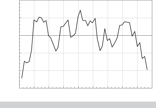
20.9.2 APPLICATION: ESTIMATION OF A MODEL
WITH AUTOCORRELATION
The model of the U.S. gasoline market that appears in Example 6.9 is
ln
G
t
pop
t
= β
1
+ β
2
ln
I
t
pop
t
+ β
3
ln P
G,t
+ β
4
ln P
NC,t
+ β
5
ln P
UC,t
+ β
6
t + ε
t
.
The results in Figure 20.2 suggest that the specification may be incomplete, and, if so,
there may be autocorrelation in the disturbances in this specification. Least squares
estimates of the parameters using the data in Appendix Table F2.2 appear in the first
row of Table 20.2. [The dependent variable is ln(Gas expenditure /(price × popula-
tion)). These are the OLS results reported in Example 6.9.] The first five autocorre-
lations of the least squares residuals are 0.667, 0.438, 0.142, −0.018, and −0.198. This
produces Box–Pierce and Box–Ljung statistics of 36.217 and 38.789, respectively, both
of which are larger than the critical value from the chi-squared table of 11.07. We
regressed the least squares residuals on the independent variables and five lags of
TABLE 20.2
Parameter Estimates (standard errors in parentheses)
β
1
β
2
β
3
β
4
β
5
β
6
ρ
OLS −26.68 1.6250 −0.05392 −0.0834 −0.08467 −0.01393 0.0000
R
2
= 0.96493 (2.000) (0.1952) (0.04216) (0.1765) (0.1024) (0.00477) (0.0000)
Prais– −18.58 0.7447 −0.1138 −0.1364 −0.008956 0.006689 0.9567
Winsten (1.768)(0.1761) (0.03689) (0.1528) (0.07213) (0.004974) (0.04078)
Cochrane– −18.76 0.7300 −0.1080 −0.06675 0.04190 −0.0001653 0.9695
Orcutt (1.382) (0.1377) (0.02885) (0.1201) (0.05713) (0.004082) (0.03434)
Maximum −16.25 0.4690 −0.1387 −0.09682 −0.001485 0.01280 0.9792
Likelihood (1.391) (0.1350) (0.02794) (0.1270) (0.05198) (0.004427) (0.02816)
AR(2) −19.45 0.8116 −0.09538 −0.09099 0.04091 −0.
001374 0.8610
(1.495) (0.1502) (0.03117) (0.1297) (0.06558) (0.004227) (0.07053)
928
PART V
✦
Time Series and Macroeconometrics
0.150
0.100
0.050
0.000
0.050
0.100
1952 1958 1964 1970 1976 1982 1988 1994 2000 2006
Residual
Year
FIGURE 20.4
Least Squares Residuals.
the residuals. (The missing values in the first five years were filled with zeros.) The
coefficients on the lagged residuals and the associated t statistics are 0.741 (4.635),
0.153 (0.789), −0.246 (−1.262), 0.0942(0.472), and −0.125 (−0.658).TheR
2
in this re-
gression is 0.549086, which produces a chi-squared value of 28.55. This is larger than
the critical value of 11.07, so once again, the null hypothesis of zero autocorrelation is
rejected. Finally, the Durbin–Watson statistic is 0.425007. For 5 regressors and 52 obser-
vations, the critical value of d
L
is 1.36, so on this basis as well, the null hypothesis ρ = 0
would pe rejected. The plot of the residuals shown in Figure 20.4 seems consistent with
this conclusion.
The Prais and Winsten FGLS estimates appear in the second row of Table 20.2
followed by the Cochrane and Orcutt results then the maximum likelihood estimates.
[The autocorrelation coefficient computed using (1−d/2) (see Section 20.7.3) is 0.78750.
The MLE is computed using the Beach and MacKinnon algorithm. See Section 14.9.2.b.]
Finally, we fit the AR(2) model by first regressing the least squares residuals, e
t
,one
t−1
and e
t−2
(without a constant term and filling the first two observations with zeros). The
two estimates are 0.751941 and −0.022464, respectively. With the estimates of θ
1
and θ
2
,
we transformed the data using y
∗
t
= y
t
−θ
1
y
t−1
−θ
2
y
t−2
and likewise for each regressor.
Two observations are then discarded, so the AR(2) regression uses 50 observations
while the Prais–Winsten estimator uses 52 and the Cochrane–Orcutt regression uses 51.
In each case, the autocorrelation of the FGLS residuals is computed and reported in
the last column of the table.
One might want to examine the residuals after estimation to ascertain whether the
AR(1) model is appropriate. In the results just presented, there are two large autocorre-
lation coefficients listed with the residual based tests, and in computing the LM statistic,
we found that the first two coefficients were statistically significant. If the AR(1) model
is appropriate, then one should find that only the coefficient on the first lagged residual