Greene W.H. Econometric Analysis

Подождите немного. Документ загружается.

CHAPTER 19

✦

Limited Dependent Variables

899

Finally, the issue of sample selection arises when the observed data are not drawn

randomly from the population of interest. Failure to account for this nonrandom sam-

pling produces a model that describes only the nonrandom subsample, not the larger

population. In each case, we examined the model speciﬁcation and estimation tech-

niques which are appropriate for these variations of the regression model. Maximum

likelihood is usually the method of choice, but for the third case, a two-step estimator

has become more common. The leading contemporary application of selection meth-

ods and endogenous sampling is in the measure of treatment effects. We considered

three approaches to analysis of treatment effects; regression methods, propensity score

matching, and regression discontinuity.

Key Terms and Concepts

•

Accelerated failure time

model

•

Attenuation

•

Average treatment effect

•

Average treatment effect on

the treated

•

Censored regression model

•

Censored variable

•

Censoring

•

Conditional mean

assumption

•

Conditional moment test

•

Control function

•

Corner solution model

•

Data envelopment analysis

•

Degree of truncation

•

Delta method

•

Difference in differences

•

Duration model

•

Exponential

•

Exponential model

•

Fuzzy design

•

Generalized residual

•

Hazard function

•

Hazard rate

•

Heterogeneity

•

Heteroscedasticity

•

Hurdle model

•

Incidental truncation

•

Instrumetal variable

estimation

•

Integrated hazard function

•

Inverse probability

weighted estimator

•

Inverse Mills ratio

•

Lagrange multiplier test

•

Matching estimator

•

Mean independence

assumption

•

Missing counterfactual

•

Negative duration

dependence

•

Olsen’s reparameterization

•

Parametric

•

Parametric model

•

Partial likelihood

•

Positive duration

dependence

•

Product limit estimator

•

Propensity score

•

Proportional hazard

•

Regression discontinuity

design

•

Risk set

•

Rubin causal model

•

Sample selection

•

Selection on observables

•

Selection on unobservables

•

Semiparametric estimator

•

Semiparametric model

•

Speciﬁcation error

•

Stochastic frontier model

•

Survival function

•

Time-varying covariate

•

Tobit model

•

Treatment effect

•

Truncated distribution

•

Truncated mean

•

Truncated normal

distribution

•

Truncated random variable

•

Truncated standard normal

distribution

•

Truncated variance

•

Truncation

•

Two-step estimation

•

Type II tobit model

•

Weibull model

•

Weibull survival model

Exercises

1. The following 20 observations are drawn from a censored normal distribution:

3.8396 7.2040 0.00000 0.00000 4.4132 8.0230

5.7971 7.0828 0.00000 0.80260 13.0670 4.3211

0.00000 8.6801 5.4571 0.00000 8.1021 0.00000

1.2526 5.6016

900

PART IV

✦

Cross Sections, Panel Data, and Microeconometrics

The applicable model is

∗

= μ + ε

= y

∗

if μ + ε

> 0, 0 otherwise,

∼ N[0,σ

Exercises 1 through 4 in this section are based on the preceding information. The

OLS estimator of μ in the context of this tobit model is simply the sample mean.

Compute the mean of all 20 observations. Would you expect this estimator to over-

or underestimate μ? If we consider only the nonzero observations, then the trun-

cated regression model applies. The sample mean of the nonlimit observations

is the least squares estimator in this context. Compute it and then comment on

whether this sample mean should be an overestimate or an underestimate of the true

mean.

2. We now consider the tobit model that applies to the full data set.

a. Formulate the log-likelihood for this very simple tobit model.

b. Reformulate the log-likelihood in terms of θ = 1/σ and γ = μ/σ . Then derive

the necessary conditions for maximizing the log-likelihood with respect to θ

and γ .

c. Discuss how you would obtain the values of θ and γ to solve the problem in

part b.

d. Compute the maximum likelihood estimates of μ and σ .

3. Using only the nonlimit observations, repeat Exercise 2 in the context of the trun-

cated regression model. Estimate μ and σ by using the method of moments esti-

mator outlined in Example 19.2. Compare your results with those in the previous

exercises.

4. Continuing to use the data in Exercise 1, consider once again only the nonzero

observations. Suppose that the sampling mechanism is as follows: y

∗

and another

normally distributed random variable z have population correlation 0.7. The two

variables, y

∗

and z, are sampled jointly. When z is greater than zero, y is re-

ported. When z is less than zero, both z and y are discarded. Exactly 35 draws

were required to obtain the preceding sample. Estimate μ and σ. (Hint: Use Theo-

rem 19.5.)

5. Derive the partial effects for the tobit model with heteroscedasticity that is de-

scribed in Section 19.3.5.a.

6. Prove that the Hessian for the tobit model in (19-14) is negative deﬁnite after

Olsen’s transformation is applied to the parameters.

Applications

1. We examined Ray Fair’s famous analysis (Journal of Political Economy, 1978) of a

Psychology Today survey on extramarital affairs in Example 18.9 using a Poisson

regression model. Although the dependent variable used in that study was a count,

Fair (1978) used the tobit model as the platform for his study. You can reproduce

the tobit estimates in Fair’s paper easily with any software package that contains

a tobit estimator—most do. The data appear in Appendix Table F18.1. Reproduce

CHAPTER 19

✦

Limited Dependent Variables

901

Fair’s least squares and tobit estimates. Compute the partial effects for the model

and interpret all results.

2. The Mroz (1975) data used in Example 19.11 (see Appendix Table F5.1) also de-

scribe a setting in which the Tobit model has been frequently applied. The sample

contains 753 observations on labor market outcomes for married women, including

the following variables:

lfp = indicator (0/1) for whether in the formal labor market (lfp = 1)

or not (lfp = 0),

whrs = wife’s hours worked,

kl6 = number of children under 6 years old in the household,

k618 = number of children from 6 to 18 years old in the household,

wa = wife’s age,

we = wife’s education,

ww = wife’s hourly wage,

hhrs = husband’s hours worked,

ha = husband’s age,

hw = husband’s wage,

faminc = family income from other sources,

wmed = wife’s mother’s education

wfed = wife’s father’s education

cit = dummy variable for living in an urban area,

ax = labor market experience = age − we − 5,

and several variables that will not be useful here. Using these data, estimate a tobit

model for the wife’s hours worked. Report all results including partial effects and

relevant diagnostic statistics. Repeat the analysis for the wife’s labor earnings, ww

times whrs. Which is a more plausible model?

3. Continuing the analysis of the previous application, note that these data conform

precisely to the description of “corner solutions” in Section 19.3.4. The dependent

variable is not censored in the fashion usually assumed for a tobit model. To inves-

tigate whether the dependent variable is determined by a two-part decision process

(yes/no and, if yes, how much), specify and estimate a two-equation model in which

the ﬁrst equation analyzes the binary decision lfp = 1ifwhrs > 0 and 0 otherwise

and the second equation analyzes whrs |whrs > 0. What is the appropriate model?

What do you ﬁnd? Report all results.

4. StochasticFrontier Model. Section 10.5.1 presents estimates of a Cobb–Douglas

cost function using Nerlove’s 1955 data on the U.S. electric power industry. Chris-

tensen and Greene’s 1976 update of this study used 1970 data for this industry. The

Christensen and Greene data are given in Appendix Table F4.4. These data have

902

PART IV

✦

Cross Sections, Panel Data, and Microeconometrics

provided a standard test data set for estimating different forms of production and

cost functions, including the stochastic frontier model discussed in Section 19.2.4. It

has been suggested that one explanation for the apparent ﬁnding of economies of

scale in these data is that the smaller ﬁrms were inefﬁcient for other reasons. The

stochastic frontier might allow one to disentangle these effects. Use these data to

ﬁt a frontier cost function which includes a quadratic term in log output in addi-

tion to the linear term and the factor prices. Then examine the estimated Jondrow

et al. residuals to see if they do indeed vary negatively with output, as suggested.

(This will require either some programming on your part or specialized software.

The stochastic frontier model is provided as an option in Stata, TSP, and LIMDEP.

Or, the likelihood function can be programmed fairly easily for RATS, MatLab,

or GAUSS.) (Note: For a cost frontier as opposed to a production frontier, it is

necessary to reverse the sign on the argument in the  function that appears in the

log-likelihood.)

SERIAL CORRELATION

20.1 INTRODUCTION

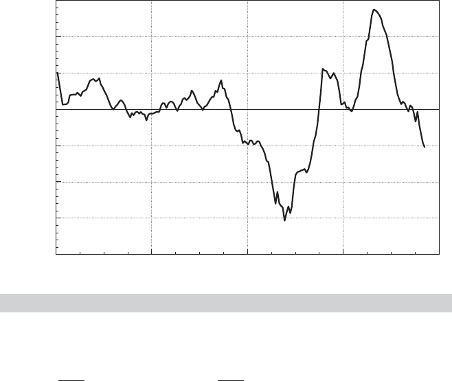
Time-series data often display autocorrelation, or serial correlation of the disturbances

across periods. Consider, for example, the plot of the least squares residuals in the

following example.

Example 20.1 Money Demand Equation

Appendix Table F5.2 contains quarterly data from 1950.1 to 2000.4 on the U.S. money stock

(M1) and output (real GDP) and the price level (CPI

U). Consider a simple (extremely) model

of money demand,

ln M1

= β

+ β

ln GDP

+ β

ln CPI

+ ε

A plot of the least squares residuals is shown in Figure 20.1. The pattern in the residuals

suggests that knowledge of the sign of a residual in one period is a good indicator of the sign of

the residual in the next period. This knowledge suggests that the effect of a given disturbance

is carried, at least in part, across periods. This sort of “memory” in the disturbances creates

the long, slow swings from positive values to negative ones that is evident in Figure 20.1. One

might argue that this pattern is the result of an obviously naive model, but that is one of the

important points in this discussion. Patterns such as this usually do not arise spontaneously;

to a large extent, they are, indeed, a result of an incomplete or ﬂawed model speciﬁcation.

One explanation for autocorrelation is that relevant factors omitted from the time-

series regression, like those included, are correlated across periods. This fact may be

due to serial correlation in factors that should be in the regression model. It is easy to

see why this situation would arise. Example 20.2 shows an obvious case.

Example 20.2 Autocorrelation Induced by Misspeciﬁcation

of the Model

In Examples 2.3, 4.2 and 4.8, we examined yearly time-series data on the U.S. gasoline market

from 1953 to 2004. The evidence in the examples was convincing that a regression model

of variation in ln G/Pop should include, at a minimum, a constant, ln P

and ln income/Pop.

Other price variables and a time trend also provide signiﬁcant explanatory power, but these

two are a bare minimum. Moreover, we also found on the basis of a Chow test of structural

change that apparently this market changed structurally after 1974. Figure 20.2 displays

plots of four sets of least squares residuals. Parts (a) through (c) show clearly that as the

speciﬁcation of the regression is expanded, the autocorrelation in the “residuals” diminishes.

Part (c) shows the effect of forcing the coefﬁcients in the equation to be the same both before

and after the structural shift. In part (d), the residuals in the two subperiods 1953 to 1974 and

1975 to 2004 are produced by separate unrestricted regressions. This latter set of residuals

is almost nonautocorrelated. (Note also that the range of variation of the residuals falls as

Because this chapter deals exclusively with time-series data, we shall use the index t for observations and T

for the sample size throughout.

903

904

PART V

✦

Time Series and Macroeconometrics

1950

0.225

0.150

0.075

0.000

0.300

0.225

0.150

0.075

1963 1976

Quarter

Residual

1989 2002

FIGURE 20.1

Autocorrelated Least Squares Residuals.

the model is improved, i.e., as its ﬁt improves.) The full equation is

Pop

= β

+ β

ln P

+ β

Pop

+ β

ln P

NCt

+ β

ln P

UCt

+β

ln P

PT t

+ β

ln P

+ β

ln P

+ β

ln P

+ β

t + ε

Finally, we consider an example in which serial correlation is an anticipated part of the

model.

Example 20.3 Negative Autocorrelation in the Phillips Curve

The Phillips curve [Phillips (1957)] has been one of the most intensively studied relationships

in the macroeconomics literature. As originally proposed, the model speciﬁes a negative re-

lationship between wage inﬂation and unemployment in the United Kingdom over a period of

100 years. Recent research has documented a similar relationship between unemployment

and price inﬂation. It is difﬁcult to justify the model when cast in simple levels; labor market

theories of the relationship rely on an uncomfortable proposition that markets persistently

fall victim to money illusion, even when the inﬂation can be anticipated. Current research

[e.g., Staiger et al. (1996)] has reformulated a short-run (disequilibrium) “expectations aug-

mented Phillips curve” in terms of unexpected inﬂation and unemployment that deviates from

a long-run equilibrium or “natural rate.” The expectations-augmented Phillips curve can

be written as

p

− E[p

|

t−1

] = β[u

− u

∗

] + ε

where p

is the rate of inﬂation in year t, E [p

|

t−1

] is the forecast of p

made in period

t − 1 based on information available at time t − 1, 

t−1

, u

is the unemployment rate and u

∗

is the natural, or equilibrium rate. (Whether u

∗

can be treated as an unchanging parameter,

as we are about to do, is controversial.) By construction, [u

− u

∗

] is disequilibrium, or cycli-

cal unemployment. In this formulation, ε

would be the supply shock (i.e., the stimulus that

produces the disequilibrium situation). To complete the model, we require a model for the

expected inﬂation. For the present, we’ll assume that economic agents are rank empiricists.

CHAPTER 20

✦

Serial Correlation

905

0.30

0.20

0.10

0.00

0.10

0.20

0.30

1952 1964 1976 1988 2000

Residual

Year

Panel

(

)

0.150

0.100

0.050

0.000

0.050

0.100

0.150

Residual

1952 1964 1976 1988 2000

Year

Panel

(

)

0.075

0.050

0.025

0.000

0.025

0.050

0.075

Residual

1952 1964 1976 1988 2000

Year

Panel (c)

0.030

0.020

0.010

0.000

0.010

0.020

0.030

Residual

1952 1964 1976 1988 2000

Year

Panel (d)

FIGURE 20.2

Unstandardized Residuals (Bars mark mean res. and

+/ − 2s(e)

The forecast of next year’s inﬂation is simply this year’s value. This produces the estimating

equation

p

− p

t−1

= β

+ β

+ ε

where β

= β and β

=−βu

∗

. Note that there is an implied estimate of the natural rate of un-

employment embedded in the equation. After estimation, u

∗

can be estimated by −b

. The

equation was estimated with the 1950.1–2000.4 data in Appendix Table F5.2 that were used

in Example 20.1 (minus two quarters for the change in the rate of inﬂation). Least squares

estimates (with standard errors in parentheses) are as follows:

p

− p

t−1

= 0.49189 − 0.090136 u

+ e

(0.7405) (0.1257) R

= 0.002561, T = 202.

The implied estimate of the natural rate of unemployment is 5.46 percent, which is in line with

other recent estimates. The estimated asymptotic covariance of b

and b

is −0.08973. Using

the delta method, we obtain a standard error of 2.2062 for this estimate, so a conﬁdence in-

terval for the natural rate is 5.46 percent ±1.96 ( 2.21 percent) = (1.13 percent, 9.79 percent)

(which seems fairly wide, but, again, whether it is reasonable to treat this as a parameter is at

least questionable). The regression of the least squares residuals on their past values gives a

slope of −0.4263 with a highly signiﬁcant t ratio of −6.725. We thus conclude that the resid-

uals (and, apparently, the disturbances) in this model are highly negatively autocorrelated.

This is consistent with the striking pattern in Figure 20.3.

906

PART V

✦

Time Series and Macroeconometrics

1950

15

10

5

1963 1976

Quarter

Residual

Phillips Curve Deviations from Expected Inflation

1989 2002

FIGURE 20.3

Negatively Autocorrelated Residuals.

The problems for estimation and inference caused by autocorrelation are similar to

(although, unfortunately, more involved than) those caused by heteroscedasticity. As

before, least squares is inefﬁcient, and inference based on the least squares estimates

is adversely affected. Depending on the underlying process, however, GLS and FGLS

estimators can be devised that circumvent these problems. There is one qualitative dif-

ference to be noted. In Section 20.13, we will examine models in which the generalized

regression model can be viewed as an extension of the regression model to the con-

ditional second moment of the dependent variable. In the case of autocorrelation, the

phenomenon arises in almost all cases from a misspeciﬁcation of the model. Views differ

on how one should react to this failure of the classical assumptions, from a pragmatic

one that treats it as another “problem” in the data to an orthodox methodological view

that it represents a major speciﬁcation issue—see, for example, “A Simple Message to

Autocorrelation Correctors: Don’t” [Mizon (1995).]

We should emphasize that the models we shall examine here are quite far removed

from the classical regression. The exact or small-sample properties of the estimators are

rarely known, and only their asymptotic properties have been derived.

20.2 THE ANALYSIS OF TIME-SERIES DATA

The treatment in this chapter will be the ﬁrst structured analysis of time-series data in

the text. Time-series analysis requires some revision of the interpretation of both data

generation and sampling that we have maintained thus far.

CHAPTER 20

✦

Serial Correlation

907

A time-series model will typically describe the path of a variable y

in terms of

contemporaneous (and perhaps lagged) factors x

, disturbances (innovations), ε

, and

its own past, y

t−1

,....For example,

= β

+ β

t−1

+ ε

The time series is a single occurrence of a random event. For example, the quarterly

series on real output in the United States from 1950 to 2000 that we examined in Ex-

ample 20.1 is a single realization of a process, GDP

. The entire history over this period

constitutes a realization of the process. At least in economics, the process could not be

repeated. There is no counterpart to repeated sampling in a cross section or replication

of an experiment involving a time-series process in physics or engineering. Nonethe-

less, were circumstances different at the end of World War II, the observed history

could have been different. In principle, a completely different realization of the en-

tire series might have occurred. The sequence of observations, {y

}

t=∞

t=−∞

is a time-series

process, which is characterized by its time ordering and its systematic correlation be-

tween observations in the sequence. The signature characteristic of a time-series process

is that empirically, the data generating mechanism produces exactly one realization of

the sequence. Statistical results based on sampling characteristics concern not random

sampling from a population, but from distributions of statistics constructed from sets

of observations taken from this realization in a time window, t =1,...,T. Asymptotic

distribution theory in this context concerns behavior of statistics constructed from an

increasingly long window in this sequence.

The properties of y

as a random variable in a cross section are straightforward

and are conveniently summarized in a statement about its mean and variance or the

probability distribution generating y

. The statement is less obvious here. It is common

to assume that innovations are generated independently from one period to the next,

with the familiar assumptions

E [ε

] = 0,

Var[ε

] = σ

and

Cov[ε

,ε

] = 0 for t = s.

In the current context, this distribution of ε

is said to be covariance stationary or

weakly stationary. Thus, although the substantive notion of “random sampling” must

be extended for the time series ε

, the mathematical results based on that notion apply

here. It can be said, for example, that ε

is generated by a time-series process whose

mean and variance are not changing over time. As such, by the method we will discuss

in this chapter, we could, at least in principle, obtain sample information and use it to

characterize the distribution of ε

. Could the same be said of y

? There is an obvious

difference between the series ε

and y

; observations on y

at different points in time

are necessarily correlated. Suppose that the y

series is weakly stationary and that, for

the moment, β

= 0. Then we could say that

E [y

] = β

+ β

E [y

t−1

] + E [ε

] = β

/(1 − β

)

and

Var[y

] = β

Var[y

t−1

] + Var[ε

908

PART V

✦

Time Series and Macroeconometrics

= β

+ σ

so that

1 − β

Thus, γ

, the variance of y

, is a ﬁxed characteristic of the process generating y

. Note

how the stationarity assumption, which apparently includes |β

|< 1, has been used. The

assumption that |β

|< 1 is needed to ensure a ﬁnite and positive variance.

Finally, the

same results can be obtained for nonzero β

if it is further assumed that x

is a weakly

stationary series.

Alternatively, consider simply repeated substitution of lagged values into the ex-

pression for y

= β

+ β

(β

+ β

t−2

+ ε

t−1

) + ε

(20-1)

and so on. We see that, in fact, the current y

is an accumulation of the entire history of

the innovations, ε

. So if we wish to characterize the distribution of y

, then we might

do so in terms of sums of random variables. By continuing to substitute for y

t−2

, then

t−3

,...in (20-1), we obtain an explicit representation of this idea,

∞



i=0

(β

+ ε

t−i

Do sums that reach back into inﬁnite past make any sense? We might view the

process as having begun generating data at some remote, effectively “inﬁnite” past. As

long as distant observations become progressively less important, the extension to an

inﬁnite past is merely a mathematical convenience. The diminishing importance of past

observations is implied by |β

|< 1. Notice that, not coincidentally, this requirement is

the same as that needed to solve for γ

in the preceding paragraphs. A second possibility

is to assume that the observation of this time series begins at some time 0 [with (x

,ε

)

called the initial conditions], by which time the underlying process has reached a state

such that the mean and variance of y

are not (or are no longer) changing over time. The

mathematics are slightly different, but we are led to the same characterization of the

random process generating y

. In fact, the same weak stationarity assumption ensures

both of them.

Except in very special cases, we would expect all the elements in the T component

random vector (y

,...,y

) to be correlated. In this instance, said correlation is called

“autocorrelation.” As such, the results pertaining to estimation with independent or

uncorrelated observations that we used in the previous chapters are no longer usable.

In point of fact, we have a sample of but one observation on the multivariate random

variable [y

, t = 1,...,T]. There is a counterpart to the cross-sectional notion of pa-

rameter estimation, but only under assumptions (e.g., weak stationarity) that establish

that parameters in the familiar sense even exist. Even with stationarity, it will emerge

The current literature in macroeconometrics and time series analysis is dominated by analysis of cases in

which β

= 1 (or counterparts in different models). We will return to this subject in Chapter 21.

See Section 20.4.1 on the stationarity assumption.