Greene W.H. Econometric Analysis

Подождите немного. Документ загружается.

CHAPTER 21

✦

Nonstationary Data

959

with it. Comparing these results to the values in Table 21.4 we conclude (again) that there is,

indeed, a unit root in In GDP. Or, more precisely, we conclude that In GDP is not a stationary

series, nor even a trend stationary series.

21.3 COINTEGRATION

Studies in empirical macroeconomics almost always involve nonstationary and trending

variables, such as income, consumption, money demand, the price level, trade ﬂows, and

exchange rates. Accumulated wisdom and the results of the previous sections suggest

that the appropriate way to manipulate such series is to use differencing and other

transformations (such as seasonal adjustment) to reduce them to stationarity and then to

analyze the resulting series as VARs or with the methods of Box and Jenkins. But recent

research and a growing literature has shown that there are more interesting, appropriate

ways to analyze trending variables.

In the fully speciﬁed regression model

= βx

+ ε

there is a presumption that the disturbances ε

are a stationary, white noise series.

But this presumption is unlikely to be true if y

and x

are integrated series. Generally,

if two series are integrated to different orders, then linear combinations of them will

be integrated to the higher of the two orders. Thus, if y

and x

are I(1)—that is, if both

are trending variables—then we would normally expect y

− β x

to be I (1) regardless

of the value of β, not I(0) (i.e., not stationary). If y

and x

are each drifting upward

with their own trend, then unless there is some relationship between those trends, the

difference between them should also be growing, with yet another trend. There must

be some kind of inconsistency in the model. On the other hand, if the two series are

both I (1), then there may be a β such that

= y

− βx

is I (0). Intuitively, if the two series are both I(1), then this partial difference between

them might be stable around a ﬁxed mean. The implication would be that the series are

drifting together at roughly the same rate. Two series that satisfy this requirement are

said to be cointegrated, and the vector [1, −β] (or any multiple of it) is a cointegrating

vector. In such a case, we can distinguish between a long-run relationship between y

and x

, that is, the manner in which the two variables drift upward together, and the

short-run dynamics, that is, the relationship between deviations of y

from its long-run

trend and deviations of x

from its long-run trend. If this is the case, then differencing of

the data would be counterproductive, since it would obscure the long-run relationship

between y

and x

. Studies of cointegration and a related technique, error correction,

are concerned with methods of estimation that preserve the information about both

forms of covariation.

If there is autocorrelation in the model, then it has been removed through an appropriate transformation.

See, for example, Engle and Granger (1987) and the lengthy literature cited in Hamilton (1994). A survey

paper on VARs and cointegration is Watson (1994).

960

PART V

✦

Time Series and Macroeconometrics

1949

6.6

7.2

Quarter

Logs

1962 1975 20011988

7.8

8.4

9.0

9.6

LOGGDP

LOGCONS

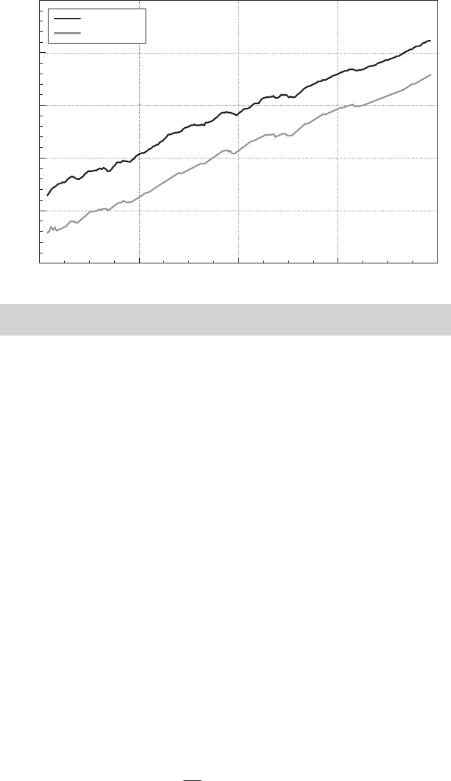
FIGURE 21.10

Cointegrated Variables: Logs of Consumption

and GDP.

Example 21.5 Cointegration in Consumption and Output

Consumption and income provide one of the more familiar examples of the phenomenon

described previously. The logs of GDP and consumption for 1950.1 to 2000.4 are plotted

in Figure 21.10. Both variables are obviously nonstationary. We have already veriﬁed that

there is a unit root in the income data. We leave as an exercise for the reader to verify that

the consumption variable is likewise I (1) . Nonetheless, there is a clear relationship between

consumption and output. To see where this discussion of relationships among variables

is going, consider a simple regression of the log of consumption on the log of income,

where both variables are manipulated in mean deviation form (so, the regression includes

a constant). The slope in that regression is 1.056765. The residuals from the regression,

= [lnCons

∗

, lnGDP

∗

][1, −1.056765]



(where the “

∗

” indicates mean deviations) are plotted

in Figure 21.11. The trend is clearly absent from the residuals. But, it remains to verify whether

the series of residuals is stationary. In the ADF regression of the least squares residuals

on a constant (random walk with drift), the lagged value and the lagged ﬁrst difference,

the coefﬁcient on u

t−1

is 0.838488 (0.0370205) and that on u

t−1

− u

t−2

is −0.098522. (The

constant differs trivially from zero because two observations are lost in computing the ADF

regression.) With 202 observations, we ﬁnd DF

=−4.63 and DF

=−29.55. Both are well

below the critical values, which suggests that the residual series does not contain a unit

root. We conclude (at least it appears so) that even after accounting for the trend, although

neither of the original variables is stationary, there is a linear combination of them that is. If

this conclusion holds up after a more formal treatment of the testing procedure, we will state

that logGDP and log consumption are cointegrated.

Example 21.6 Several Cointegrated Series

The theory of purchasing power parity speciﬁes that in long-run equilibrium, exchange rates

will adjust to erase differences in purchasing power across different economies. Thus, if p

and p

are the price levels in two countries and E is the exchange rate between the two

currencies, then in equilibrium,

= E

= μ, a constant.

CHAPTER 21

✦

Nonstationary Data

961

1950

0.050

0.025

Quarter

Residual

1963 1976 20021989

0.000

0.025

0.050

0.075

FIGURE 21.11

Residuals from Consumption—Income Regression.

The price levels in any two countries are likely to be strongly trended. But allowing for short-

term deviations from equilibrium, the theory suggests that for a particular β = (lnμ, −1, 1) ,

in the model

ln E

= β

+ β

ln p

+ β

ln p

+ ε

= ln v

would be a stationary series, which would imply that the logs of the three variables

in the model are cointegrated.

We suppose that the model involves M variables, y

= [y

,...,y

]



, which indi-

vidually may be I (0) or I (1), and a long-run equilibrium relationship,



γ − x



β = 0.

The “regressors” may include a constant, exogenous variables assumed to be I(0),

and/or a time trend. The vector of parameters γ is the cointegrating vector. In the short

run, the system may deviate from its equilibrium, so the relationship is rewritten as



γ − x



β = ε

where the equilibrium error ε

must be a stationary series. In fact, because there are M

variables in the system, at least in principle, there could be more than one cointegrating

vector. In a system of M variables, there can only be up to M − 1 linearly independent

cointegrating vectors. A proof of this proposition is very simple, but useful at this point.

Proof: Suppose that γ

is a cointegrating vector and that there are M linearly

independent cointegrating vectors. Then, neglecting x



β for the moment, for

every γ

, y



is a stationary series ν

. Any linear combination of a set of sta-

tionary series is stationary, so it follows that every linear combination of the

cointegrating vectors is also a cointegrating vector. If there are M such M × 1

962

PART V

✦

Time Series and Macroeconometrics

linearly independent vectors, then they form a basis for the M-dimensional

space, so any M × 1 vector can be formed from these cointegrating vectors,

including the columns of an M × M identity matrix. Thus, the ﬁrst column of

an identity matrix would be a cointegrating vector, or y

is I(0). This result is a

contradiction, because we are allowing y

to be I(1). It follows that there can

be at most M − 1 cointegrating vectors.

The number of linearly independent cointegrating vectors that exist in the equilib-

rium system is called its cointegrating rank. The cointegrating rank may range from 1 to

M − 1. If it exceeds one, then we will encounter an interesting identiﬁcation problem.

As a consequence of the observation in the preceding proof, we have the unfortunate

result that, in general, if the cointegrating rank of a system exceeds one, then without

out-of-sample, exact information, it is not possible to estimate behavioral relationships

as cointegrating vectors. Enders (1995) provides a useful example.

Example 21.7 Multiple Cointegrating Vectors

We consider the logs of four variables, money demand m, the price level p, real income y,

and an interest rate r . The basic relationship is

m = γ

+ γ

p + γ

y + γ

r + ε.

The price level and real income are assumed to be I ( 1). The existence of long-run equilibrium

in the money market implies a cointegrating vector α

. If the Fed follows a certain feedback

rule, increasing the money stock when nominal income ( y + p) is low and decreasing it when

nominal income is high—which might make more sense in terms of rates of growth—then

there is a second cointegrating vector in which γ

= γ

and γ

= 0. Suppose that we label

this vector α

. The parameters in the money demand equation, notably the interest elasticity,

are interesting quantities, and we might seek to estimate α

to learn the value of this quantity.

But since every linear combination of α

and α

is a cointegrating vector, to this point we are

only able to estimate a hash of the two cointegrating vectors.

In fact, the parameters of this model are identiﬁable from sample information (in principle).

We have speciﬁed two cointegrating vectors,

= [1, −γ

, −γ

]

and

= [1, −γ

, γ

,0]



Although it is true that every linear combination of α

and α

is a cointegrating vector, only

the original two vectors, as they are, have a 1 in the ﬁrst position of both anda0inthe

last position of the second. (The equality restriction actually overidentiﬁes the parameter

matrix.) This result is, of course, exactly the sort of analysis that we used in establishing the

identiﬁability of a simultaneous equations system.

21.3.1 COMMON TRENDS

If two I(1) variables are cointegrated, then some linear combination of them is I (0).

Intuition should suggest that the linear combination does not mysteriously create a

well-behaved new variable; rather, something present in the original variables must be

missing from the aggregated one. Consider an example. Suppose that two I(1) variables

have a linear trend,

= α + βt + u

= γ + δt + v

CHAPTER 21

✦

Nonstationary Data

963

where u

and v

are white noise. A linear combination of y

and y

with vector (1,θ)

produces the new variable,

= (α + θγ) + (β +θδ)t + u

+ θv

which, in general, is still I(1). In fact, the only way the z

series can be made stationary

is if θ =−β/δ. If so, then the effect of combining the two variables linearly is to remove

the common linear trend, which is the basis of Stock and Watson’s (1988) analysis of the

problem. But their observation goes an important step beyond this one. The only way

that y

and y

can be cointegrated to begin with is if they have a common trend of some

sort. To continue, suppose that instead of the linear trend t, the terms on the right-hand

side, y

and y

, are functions of a random walk, w

= w

t−1

+η

, where η

is white noise.

The analysis is identical. But now suppose that each variable y

has its own random

walk component w

, i = 1, 2. Any linear combination of y

and y

must involve both

random walks. It is clear that they cannot be cointegrated unless, in fact, w

= w

That is, once again, they must have a common trend. Finally, suppose that y

and y

share two common trends,

= α + βt + λw

+ u

= γ + δt + πw

+ v

We place no restriction on λ and π . Then, a bit of manipulation will show that it is not

possible to ﬁnd a linear combination of y

and y

that is cointegrated, even though

they share common trends. The end result for this example is that if y

and y

are

cointegrated, then they must share exactly one common trend.

As Stock and Watson determined, the preceding is the crux of the cointegration

of economic variables. A set of M variables that are cointegrated can be written as a

stationary component plus linear combinations of a smaller set of common trends. If

the cointegrating rank of the system is r, then there can be up to M −r linear trends

and M −r common random walks. [See Hamilton (1994, p. 578).] (The two-variable

case is special. In a two-variable system, there can be only one common trend in total.)

The effect of the cointegration is to purge these common trends from the resultant

variables.

21.3.2 ERROR CORRECTION AND VAR REPRESENTATIONS

Suppose that the two I(1) variables y

and z

are cointegrated and that the cointegrating

vector is [1, −θ]. Then all three variables, y

= y

− y

t−1

,z

, and (y

− θ z

) are I(0).

The error correction model

y

= x



β + γ(z

) + λ(y

t−1

− θ z

t−1

) + ε

describes the variation in y

around its long-run trend in terms of a set of I(0) exogenous

factors x

, the variation of z

around its long-run trend, and the error correction (y

−θ z

which is the equilibrium error in the model of cointegration. There is a tight connection

between models of cointegration and models of error correction. The model in this form

is reasonable as it stands, but in fact, it is only internally consistent if the two variables

are cointegrated. If not, then the third term, and hence the right-hand side, cannot be

I(0), even though the left-hand side must be. The upshot is that the same assumption

that we make to produce the cointegration implies (and is implied by) the existence

964

PART V

✦

Time Series and Macroeconometrics

of an error correction model.

As we will examine in the next section, the utility of

this representation is that it suggests a way to build an elaborate model of the long-run

variation in y

as well as a test for cointegration. Looking ahead, the preceding suggests

that residuals from an estimated cointegration model—that is, estimated equilibrium

errors—can be included in an elaborate model of the long-run covariation of y

and

. Once again, we have the foundation of Engel and Granger’s approach to analyzing

cointegration.

Pesaran, Shin, and Smith (2001) suggest a method of testing for a relationship in

levels between a y

and x

when there exits signiﬁcant lags in the error correction form.

Their bounds test accommodates the possibility that the regressors may be trend or

difference stationary. The critical values they provide give a band that covers the polar

cases in which all regressors are I(0), or are I(1), or are mutually cointegrated. The

statistic is able to test for the existence of a levels equation regardless of whether the

variables are I (0), I(1), or are cointegrated. In their application, y

is real earnings in

the UK while x

includes a measure of productivity, the unemployment rate, union-

ization of the workforce, a “replacement ratio” that measures the difference between

unemployment beneﬁts and real wages, and a “wedge” between the real product wage

and the real consumption wage. It is found that wages and productivity have unit roots.

The issue then is to discern whether unionization, the wedge, and the unemployment

rate, which might be I(0), have level effects in the model.

Consider the VAR representation of the model

= y

t−1

+ ε

where the vector y

is [y

, z

]



. Now take ﬁrst differences to obtain

− y

t−1

= ( − I)y

t−1

+ ε

y

= y

t−1

+ ε

If all variables are I (1), then all M variables on the left-hand side are I (0). Whether

those on the right-hand side are I (0) remains to be seen. The matrix  produces linear

combinations of the variables in y

. But as we have seen, not all linear combinations

can be cointegrated. The number of such independent linear combinations is r < M.

Therefore, although there must be a VAR representation of the model, cointegration

implies a restriction on the rank of . It cannot have full rank; its rank is r . From another

viewpoint, a different approach to discerning cointegration is suggested. Suppose that

we estimate this model as an unrestricted VAR. The resultant coefﬁcient matrix should

be short-ranked. The implication is that if we ﬁt the VAR model and impose short rank

on the coefﬁcient matrix as a restriction—how we could do that remains to be seen—

then if the variables really are cointegrated, this restriction should not lead to a loss

of ﬁt. This implication is the basis of Johansen’s (1988) and Stock and Watson’s (1988)

analysis of cointegration.

The result in its general form is known as the Granger representation theorem. See Hamilton (1994, p. 582).

CHAPTER 21

✦

Nonstationary Data

965

21.3.3 TESTING FOR COINTEGRATION

A natural ﬁrst step in the analysis of cointegration is to establish that it is indeed a

characteristic of the data. Two broad approaches for testing for cointegration have

been developed. The Engle and Granger (1987) method is based on assessing whether

single-equation estimates of the equilibrium errors appear to be stationary. The second

approach, due to Johansen (1988, 1991) and Stock and Watson (1988), is based on

the VAR approach. As noted earlier, if a set of variables is truly cointegrated, then

we should be able to detect the implied restrictions in an otherwise unrestricted VAR.

We will examine these two methods in turn.

Let y

denote the set of M variables that are believed to be cointegrated. Step one of

either analysis is to establish that the variables are indeed integrated to the same order.

The Dickey–Fuller tests discussed in Section 21.2.4 can be used for this purpose. If the

evidence suggests that the variables are integrated to different orders or not at all, then

the speciﬁcation of the model should be reconsidered.

If the cointegration rank of the system is r , then there are r independent vectors,

= [1, −θ

], where each vector is distinguished by being normalized on a different

variable. If we suppose that there are also a set of I(0) exogenous variables, includ-

ing a constant, in the model, then each cointegrating vector produces the equilibrium

relationship



= x



β + ε

which we may rewrite as

= Y



+ x



β + ε

We can obtain estimates of θ

by least squares regression. If the theory is correct and if

this OLS estimator is consistent, then residuals from this regression should estimate the

equilibrium errors. There are two obstacles to consistency. First, because both sides of

the equation contain I(1) variables, the problem of spurious regressions appears. Sec-

ond, a moment’s thought should suggest that what we have done is extract an equation

from an otherwise ordinary simultaneous equations model and propose to estimate its

parameters by ordinary least squares. As we examined in Chapter 10, consistency is

unlikely in that case. It is one of the extraordinary results of this body of theory that in

this setting, neither of these considerations is a problem. In fact, as shown by a number

of authors [see, e.g., Davidson and MacKinnon (1993)], not only is c

, the OLS estimator

of θ

, consistent, it is superconsistent in that its asymptotic variance is O(1/T

) rather

than O(1/T ) as in the usual case. Consequently, the problem of spurious regressions

disappears as well. Therefore, the next step is to estimate the cointegrating vector(s),

by OLS. Under all the assumptions thus far, the residuals from these regressions, e

are estimates of the equilibrium errors, ε

. As such, they should be I(0). The natural

approach would be to apply the familiar Dickey–Fuller tests to these residuals. The

logic is sound, but the Dickey–Fuller tables are inappropriate for these estimated er-

rors. Estimates of the appropriate critical values for the tests are given by Engle and

Granger (1987), Engle and Yoo (1987), Phillips and Ouliaris (1990), and Davidson and

MacKinnon (1993). If autocorrelation in the equilibrium errors is suspected, then an

augmented Engle and Granger test can be based on the template

e

= δe

i,t−1

+ φ

(e

i,t−1

) +···+u

966

PART V

✦

Time Series and Macroeconometrics

If the null hypothesis that δ = 0 cannot be rejected (against the alternative δ<0), then

we conclude that the variables are not cointegrated. (Cointegration can be rejected by

this method. Failing to reject does not conﬁrm it, of course. But having failed to reject

the presence of cointegration, we will proceed as if our ﬁnding had been afﬁrmative.)

Example 21.8 (Continued) Cointegration in Consumption and Output

In the example presented at the beginning of this discussion, we proposed precisely the sort

of test suggested by Phillips and Ouliaris (1990) to determine if (log) consumption and (log)

GDP are cointegrated. As noted, the logic of our approach is sound, but a few considerations

remain. The Dickey–Fuller critical values suggested for the test are appropriate only in a few

cases, and not when several trending variables appear in the equation. For the case of only

a pair of trended variables, as we have here, one may use inﬁnite sample values in the

Dickey–Fuller tables for the trend stationary form of the equation. (The drift and trend would

have been removed from the residuals by the original regression, which would have these

terms either embedded in the variables or explicitly in the equation.) Finally, there remains an

issue of how many lagged differences to include in the ADF regression. We have speciﬁed

one, although further analysis might be called for. [A lengthy discussion of this set of issues

appears in Hayashi (2000, pp. 645–648).] Thus, but for the possibility of this speciﬁcation

issue, the ADF approach suggested in the introduction does pass muster. The sample value

found earlier was −4.63. The critical values from the table are −3.45 for 5 percent and −3.67

for 2.5 percent. Thus, we conclude (as have many other analysts) that log consumption and

log GDP are cointegrated.

The Johansen (1988, 1992) and Stock and Watson (1988) methods are similar, so

we will describe only the ﬁrst one. The theory is beyond the scope of this text, although

the operational details are suggestive. To carry out the Johansen test, we ﬁrst formulate

the VAR:

= 

t−1

+ 

t−2

+···+

t−p

+ ε

The order of the model, p, must be determined in advance. Now, let z

denote the vector

of M(p − 1) variables,

= [y

t−1

,y

t−2

,...,y

t−p+1

That is, z

contains the lags 1 to p−1 of the ﬁrst differences of all M variables. Now, using

the T available observations, we obtain two T × M matrices of least squares residuals:

D = the residuals in the regressions of y

on z

E = the residuals in the regressions of y

t−p

on z

We now require the M

canonical correlations between the columns in D and those

in E. To continue, we will digress brieﬂy to deﬁne the canonical correlations. Let d

∗

denote a linear combination of the columns of D, and let e

∗

denote the same from

E. We wish to choose these two linear combinations so as to maximize the correlation

between them. This pair of variables are the ﬁrst canonical variates, and their correlation

∗

is the ﬁrst canonical correlation. In the setting of cointegration, this computation has

some intuitive appeal. Now, with d

∗

and e

∗

in hand, we seek a second pair of variables d

∗

and e

∗

to maximize their correlation, subject to the constraint that this second variable

in each pair be orthogonal to the ﬁrst. This procedure continues for all M pairs of

variables. It turns out that the computation of all these is quite simple. We will not need

to compute the coefﬁcient vectors for the linear combinations. The squared canonical

CHAPTER 21

✦

Nonstationary Data

967

correlations are simply the ordered characteristic roots of the matrix

∗

= R

−1/2

−1

−1/2

where R

is the (cross-) correlation matrix between variables in set i and set j, for

i, j = D, E.

Finally, the null hypothesis that there are r or fewer cointegrating vectors is tested

using the test statistic

TRACE TEST =−T



i=r+1

ln[1 − (r

∗

)

If the correlations based on actual disturbances had been observed instead of esti-

mated, then we would refer this statistic to the chi-squared distribution with M − r

degrees of freedom. Alternative sets of appropriate tables are given by Johansen and

Juselius (1990) and Osterwald-Lenum (1992). Large values give evidence against the

hypothesis of r or fewer cointegrating vectors.

21.3.4 ESTIMATING COINTEGRATION RELATIONSHIPS

Both of the testing procedures discussed earlier involve actually estimating the coin-

tegrating vectors, so this additional section is actually superﬂuous. In the Engle and

Granger framework, at a second step after the cointegration test, we can use the resid-

uals from the static regression as an error correction term in a dynamic, ﬁrst-difference

regression, as shown in Section 21.3.2. One can then “test down” to ﬁnd a satisfactory

structure. In the Johansen test shown earlier, the characteristic vectors corresponding to

the canonical correlations are the sample estimates of the cointegrating vectors. Once

again, computation of an error correction model based on these ﬁrst step results is a

natural next step. We will explore these in an application.

21.3.5 APPLICATION: GERMAN MONEY DEMAND

The demand for money has provided a convenient and well targeted illustration of

methods of cointegration analysis. The central equation of the model is

− p

= μ + βy

+ γ i

+ ε

, (21-8)

where m

, p

, and y

are the logs of nominal money demand, the price level, and output,

and i is the nominal interest rate (not the log of). The equation involves trending

variables (m

, p

, y

), and one that we found earlier appears to be a random walk with

drift (i

). As such, the usual form of statistical inference for estimation of the income

elasticity and interest semielasticity based on stationary data is likely to be misleading.

Beyer (1998) analyzed the demand for money in Germany over the period 1975

to 1994. A central focus of the study was whether the 1990 reuniﬁcation produced a

structural break in the long-run demand function. (The analysis extended an earlier

study by the same author that was based on data that predated the reuniﬁcation.) One

of the interesting questions pursued in this literature concerns the stability of the long-

term demand equation,

(m − p)

− y

= μ + γ i

+ ε

. (21-9)

968

PART V

✦

Time Series and Macroeconometrics

TABLE 21.6

Augmented Dickey–Fuller Tests for Variables in the Beyer Model

Variable m m 

mp p 

p 

p 

Spec. TS RW RW TS RW/D RW RW/D RW

lag 04 343 22 2

−1.82 −1.61 −6.87 −2.09 −2.14 −10.6 −2.66 −5.48

Crit. Value −3.47 −1.95 −1.95 −3.47 −2.90 −1.95 −2.90 −1.95

Variable y yRSRS RL RL (m − p)(m − p)

Spec. TS RW/D TS RW TS RW RW/D RW/D

lag 43 101 00 0

−1.83 −2.91 −2.33 −5.26 −2.40 −6.01 −1.65 −8.50

Crit. Value −3.47 −2.90 −2.90 −1.95 −2.90 −1.95 −3.47 −2.90

The left-hand side is the log of the inverse of the velocity of money, as suggested by

Lucas (1988). An issue to be confronted in this speciﬁcation is the exogeneity of the

interest variable—exogeneity [in the Engle, Hendry, and Richard (1993) sense] of in-

come is moot in the long-run equation as its coefﬁcient is assumed (per Lucas) to equal

one. Beyer explored this latter issue in the framework developed by Engle et al. (see

Section 21.3.5).

The analytical platform of Beyer’s study is a long-run function for the real money

stock M3 (we adopt the author’s notation)

(m − p)

∗

= δ

+ δ

y + δ

RS + δ

RL + δ



p, (21-10)

where RS is a short-term interest rate, RL is a long-term interest rate, and 

p is the

annual inﬂation rate—the data are quarterly. The ﬁrst step is an examination of the

data. Augmented Dickey–Fuller tests suggest that for these German data in this period,

and p

are I (2), while (m

− p

), y

,

, RS

, and RL

are all I (1). Some of Beyer’s

results which produced these conclusions are shown in Table 21.6. Note that although

both m

and p

appear to be I(2), their simple difference (linear combination) is I(1),

that is, integrated to a lower order. That produces the long-run speciﬁcation given by

(21-10). The Lucas speciﬁcation is layered onto this to produce the model for the long-

run velocity

(m − p − y)

∗

= δ

∗

+ δ

∗

RS + δ

∗

RL + δ

∗



p. (21-11)

21.3.5.a Cointegration Analysis and a Long-Run Theoretical Model

For (21-10) to be a valid model, there must be at least one cointegrating vector that

transforms z

= [(m

− p

), y

, RS

, RL

,

] to stationarity. The Johansen trace test

described in Section 21.3.3 was applied to the VAR consisting of these ﬁve I(1) vari-

ables. A lag length of two was chosen for the analysis. The results of the trace test

are a bit ambiguous; the hypothesis that r = 0 is rejected, albeit not strongly (sample

value = 90.17 against a 95 percent critical value = 87.31) while the hypothesis that

r ≤ 1 is not rejected (sample value =60.15 against a 95 percent critical value of 62.99).

(These borderline results follow from the result that Beyer’s ﬁrst three eigenvalues—

canonical correlations in the trace test statistic—are nearly equal. Variation in the test

statistic results from variation in the correlations.) On this basis, it is concluded that the