Greene W.H. Econometric Analysis

Подождите немного. Документ загружается.

CHAPTER 4

✦

The Least Squares Estimator

THEOREM 4.5

Asymptotic Distribution of a Function of b

If f(b) is a set of continuous and continuously differentiable functions of b

such that  = ∂f(β)/∂β



and if Theorem 4.4 holds, then

f(b)

∼ N



f(β), 



−1









. (4-36)

In practice, the estimator of the asymptotic covariance matrix would be

Est. Asy. Var[f(b)] = C[s



−1



If any of the functions are nonlinear, then the property of unbiasedness that holds

for b may not carry over to f(b). Nonetheless, it follows from (4-25) that f(b)isa

consistent estimator of f(β), and the asymptotic covariance matrix is readily available.

Example 4.4 Nonlinear Functions of Parameters: The Delta Method

A dynamic version of the demand for gasoline model in Example 2.3 would be used to

separate the short- and long-term impacts of changes in income and prices. The model

would be

ln( G/Pop)

= β

+ β

In P

G,t

+ β

In(Income/Pop)

+ β

InP

nc,t

+β

In P

uc,t

+ γ ln( G/Pop)

t−1

+ ε

where P

and P

are price indexes for new and used cars. In this model, the short-run

price and income elasticities are β

and β

. The long-run elasticities are φ

= β

/(1 − γ )

and φ

= β

/(1 − γ ), respectively. To estimate the long-run elasticities, we will estimate

the parameters by least squares and then compute these two nonlinear functions of the

estimates. We can use the delta method to estimate the standard errors.

Least squares estimates of the model parameters with standard errors and t ratios are

given in Table 4.3. The estimated short-run elasticities are the estimates given in the table.

The two estimated long-run elasticities are f

= b

/(1− c) =−0.069532/(1 − 0.830971) =

−0.411358 and f

= 0.164047/(1 − 0.830971) = 0.970522. To compute the estimates of

the standard errors, we need the partial derivatives of these functions with respect to the six

parameters in the model:



= ∂φ

/∂β



= [0, 1/(1− γ ) , 0, 0, 0, β

/(1− γ )

] = [0, 5.91613, 0, 0, 0, −2.43365],



= ∂φ

/∂β



= [0, 0, 1/(1− γ ) , 0, 0, β

/(1− γ )

] = [0, 0, 5.91613, 0, 0, 5.74174].

Using (4-36), we can now compute the estimates of the asymptotic variances for the two

estimated long-run elasticities by computing g



−1

and g



−1

. The results

are 0.023194 and 0.0263692, respectively. The two asymptotic standard errors are the square

roots, 0.152296 and 0.162386.

4.4.5 ASYMPTOTIC EFFICIENCY

We have not established any large-sample counterpart to the Gauss–Markov theorem.

That is, it remains to establish whether the large-sample properties of the least squares

estimator are optimal by any measure. The Gauss–Markov theorem establishes ﬁnite

PART I

✦

The Linear Regression Model

TABLE 4.3

Regression Results for a Demand Equation

Sum of squared residuals: 0.0127352

Standard error of the regression: 0.0168227

based on 51 observations 0.9951081

Variable Coefﬁcient Standard Error t Ratio

Constant −3.123195 0.99583 −3.136

ln P

−0.069532 0.01473 −4.720

ln Income / Pop 0.164047 0.05503 2.981

ln P

−0.178395 0.05517 −3.233

ln P

0.127009 0.03577 3.551

last period ln G/Pop 0.830971 0.04576 18.158

Estimated Covariance Matrix for b (e − n = times 10

−n

)

Constant ln P

ln(Income/Pop) ln P

ln P

ln(G/Pop)

t−1

0.99168

−0.0012088 0.00021705

−0.052602 1.62165e–5 0.0030279

0.0051016 −0.00021705 −0.00024708 0.0030440

0.0091672 −4.0551e–5 −0.00060624 −0.0016782 0.0012795

0.043915 −0.0001109 −0.0021881 0.00068116 8.57001e–5 0.0020943

sample conditions under which least squares is optimal. The requirements that the es-

timator be linear and unbiased limit the theorem’s generality, however. One of the

main purposes of the analysis in this chapter is to broaden the class of estimators in

the linear regression model to those which might be biased, but which are consistent.

Ultimately, we shall also be interested in nonlinear estimators. These cases extend be-

yond the reach of the Gauss–Markov theorem. To make any progress in this direction,

we will require an alternative estimation criterion.

DEFINITION 4.1

Asymptotic Efﬁciency

An estimator is asymptotically efﬁcient if it is consistent, asymptotically normally

distributed, and has an asymptotic covariance matrix that is not larger than the

asymptotic covariance matrix of any other consistent, asymptotically normally

distributed estimator.

We can compare estimators based on their asymptotic variances. The complication

in comparing two consistent estimators is that both converge to the true parameter

as the sample size increases. Moreover, it usually happens (as in our example 4.5),

that they converge at the same rate—that is, in both cases, the asymptotic variance of

the two estimators are of the same order, such as O(1/n). In such a situation, we can

sometimes compare the asymptotic variances for the same n to resolve the ranking.

The least absolute deviations estimator as an alternative to least squares provides an

example.

CHAPTER 4

✦

The Least Squares Estimator

Example 4.5 Least Squares vs. Least Absolute Deviations—A Monte

Carlo Study

We noted earlier (Section 4.2) that while it enjoys several virtues, least squares is not the only

available estimator for the parameters of the linear regresson model. Least absolute devia-

tions (LAD) is an alternative. (The LAD estimator is considered in more detail in Section 7.3.1.)

The LAD estimator is obtained as

LAD

= the minimizer of



i =1

− x



in contrast to the linear least squares estimator, which is

= the minimizer of



i =1

( y

− x



)

Suppose the regression model is deﬁned by

= x



β + ε

where the distribution of ε

has conditional mean zero, constant variance σ

, and conditional

median zero as well—the distribution is symmetric—and plim(1/n)X



ε = 0. That is, all the

usual regression assumptions, but with the normality assumption replaced by symmetry of

the distribution. Then, under our assumptions, b

is a consistent and asymptotically normally

distributed estimator with asymptotic covariance matrix given in Theorem 4.4, which we will

call σ

A. As Koenker and Bassett (1978, 1982), Huber (1987), Rogers (1993), and Koenker

(2005) have discussed, under these assumptions, b

LAD

is also consistent. A good estimator

of the asymptotic variance of b

LAD

would be (1/2)

[1/f(0)]

A where f(0) is the density of ε

at its median, zero. This means that we can compare these two estimators based on their

asymptotic variances. The ratio of the asymptotic variance of the kth element of b

LAD

to the

corresponding element of b

would be

= Var( b

k,LAD

)/Var( b

k,LS

) = (1/2)

(1/σ

)[1/ f (0)]

If ε did actually have a normal distribution with mean (and median) zero, then

f ( ε) = (2πσ

)

−1/2

exp(−ε

/(2σ

))

so f (0) = (2πσ

)

−1/2

and for this special case q

= π/2. Thus, if the disturbances are normally

distributed, then LAD will be asymptotically less efﬁcient by a factor of π/2 = 1.573.

The usefulness of the LAD estimator arises precisely in cases in which we cannot assume

normally distributed disturbances. Then it becomes unclear which is the better estimator. It

has been found in a long body of research that the advantage of the LAD estimator is most

likely to appear in small samples and when the distribution of ε has thicker tails than the

normal — that is, when outlying values of y

are more likely. As the sample size grows larger,

one can expect the LS estimator to regain its superiority. We will explore this aspect of the

estimator in a small Monte Carlo study.

Examples 2.6 and 3.4 note an intriguing feature of the ﬁne art market. At least in some

settings, large paintings sell for more at auction than small ones. Appendix Table F4.1 contains

the sale prices, widths, and heights of 430 Monet paintings. These paintings sold at auction

for prices ranging from $10,000 up to as much as $33 million. A linear regression of the log

of the price on a constant term, the log of the surface area, and the aspect ratio produces

the results in the top line of Table 4.4. This is the focal point of our analysis. In order to study

the different behaviors of the LS and LAD estimators, we will do the following Monte Carlo

study:

We will draw without replacement 100 samples of R observations from the 430. For

each of the 100 samples, we will compute b

LS,r

and b

LAD,r

. We then compute the average of

Being a Monte Carlo study that uses a random number generator, there is a question of replicability. The

study was done with NLOGIT and is replicable. The program can be found on the Web site for the text.

The qualitative results, if not the precise numerical values, can be reproduced with other programs that allow

random sampling from a data set.

PART I

✦

The Linear Regression Model

TABLE 4.4

Estimated Equations for Art Prices

Constant Log Area Aspect Ratio

Standard Standard Standard

Full Sample Mean Deviation Mean Deviation Mean Deviation

LS −8.42653 0.61184 1.33372 0.09072 −0.16537 0.12753

LAD −7.62436 0.89055 1.20404 0.13626 −0.21260 0.13628

R = 10

LS −9.39384 6.82900 1.40481 1.00545 0.39446 2.14847

LAD −8.97714 10.24781 1.34197 1.48038 0.35842 3.04773

R = 50

LS −8.73099 2.12135 1.36735 0.30025 −0.06594 0.52222

LAD −8.91671 2.51491 1.38489 0.36299 −0.06129 0.63205

R = 100

LS −8.36163 1.32083 1.32758 0.17836 −0.17357 0.28977

LAD −8.05195 1.54190 1.27340 0.21808 −0.20700 0.29465

the 100 vectors and the sample variance of the 100 observations.

The sampling variability

of the 100 sets of results corresponds to the notion of “variation in repeated samples.” For

this experiment, we will do this for R = 10, 50, and 100. The overall sample size is fairly

large, so it is reasonable to take the full sample results as at least approximately the “true

parameters.” The standard errors reported for the full sample LAD estimator are computed

using bootstrapping. Brieﬂy, the procedure is carried out by drawing B—we used B = 100—

samples of n (430) observations with replacement, from the full sample of n observations. The

estimated variance of the LAD estimator is then obtained by computing the mean squared

deviation of these B estimates around the full sample LAD estimates (not the mean of the B

estimates). This procedure is discussed in detail in Section 15.4.

If the assumptions underlying our regression model are correct, we should observe the

following:

1. Since both estimators are consistent, the averages should resemble the preceding main

results, the more so as R increases.

2. As R increases, the sampling variance of the estimators should decline.

3. We should observe generally that the standard deviations of the LAD estimates are larger

than the corresponding values for the LS estimator.

4. When R is small, the LAD estimator should compare more favorably to the LS estimator,

but as R gets larger, the advantage of the LS estimator should become apparent.

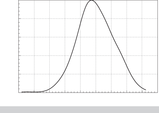
A kernel density estimate for the distribution of the least squares residuals appears in Fig-

ure 4.4. There is a bit of skewness in the distribution, so a main assumption underlying our

experiment may be violated to some degree. Results of the experiments are shown in Ta-

ble 4.4. The force of the asymptotic results can be seen most clearly in the column for the

coefﬁcient on log Area. The decline of the standard deviation as R increases is evidence of

the consistency of both estimators. In each pair of results (LS, LAD), we can also see that the

estimated standard deviation of the LAD estimator is greater by a factor of about 1.2 to 1.4,

which is also to be expected. Based on the normal distribution, we would have expected this

ratio to be

√

1.573 = 1.254.

Note that the sample size R is not a negligible fraction of the population size, 430 for each replication.

However, this does not call for a ﬁnite population correction of the variances in Table 4.4. We are not

computing the variance of a sample of R observations drawn from a population of 430 paintings. We are

computing the variance of a sample of R statistics each computed from a different subsample of the full

population. There are a bit less than 10

different samples of 10 observations we can draw. The number of

different samples of 50 or 100 is essentially inﬁnite.

CHAPTER 4

✦

The Least Squares Estimator

5

0.000

4 3 2 1 01234

0.067

0.134

0.201

Density

0.268

0.334

FIGURE 4.4

Kernel Dansity Estimator for Least Squares Residuals.

4.4.6 MAXIMUM LIKELIHOOD ESTIMATION

We have motivated the least squares estimator in two ways: First, we obtained Theorem

4.1, which states that the least squares estimator mimics the coefﬁcients in the minimum

mean squared error predictor of y in the joint distribution of y and x. Second, Theorem

4.2, the Gauss–Markov theorem, states that the least squares estimator is the minimum

variance linear unbiased estimator of β under the assumptions of the model. Neither

of these results relies on Assumption A6, normality of the distribution of ε. A natural

question at this point would be, what is the role of this assumption? There are two. First,

the assumption of normality will produce the basis for determining the appropriate

endpoints for conﬁdence intervals in Sections 4.5 and 4.6. But, we found in Section 4.4.2

that based on the central limit theorem, we could base inference on the asymptotic

normal distribution of b, even if the disturbances were not normally distributed. That

would seem to make the normality assumption no longer necessary, which is largely

true but for a second result.

If the disturbances are normally distributed, then the least squares estimator is

also the maximum likelihood estimator (MLE). We will examine maximum likelihood

estimation in detail in Chapter 14, so we will describe it only brieﬂy at this point. The

end result is that by virtue of being an MLE, least squares is asymptotically efﬁcient

among consistent and asymptotically normally distributed estimators. This is a large

sample counterpart to the Gauss–Markov theorem (known formally as the Cram´er–

Rao bound). What the two theorems have in common is that they identify the least

squares estimator as the most efﬁcient estimator in the assumed class of estimators.

They differ in the class of estimators assumed:

Gauss–Markov: Linear and unbiased estimators

ML: Based on normally distributed disturbances, consistent and asymp-

totically normally distributed estimators

PART I

✦

The Linear Regression Model

These are not “nested.” Notice, for example, that the MLE result does not require

unbiasedness or linearity. Gauss–Markov does not require normality or consistency.

The Gauss–Markov theorem is a ﬁnite sample result while the Cram´er–Rao bound

is an asymptotic (large-sample) property. The important aspect of the development

concerns the efﬁciency property. Efﬁciency, in turn, relates to the question of how best

to use the sample data for statistical inference. In general, it is difﬁcult to establish

that an estimator is efﬁcient without being speciﬁc about the candidates. The Gauss–

Markov theorem is a powerful result for the linear regression model. However, it has no

counterpart in any other modeling context, so once we leave the linear model, we will

require different tools for comparing estimators. The principle of maximum likelihood

allows the analyst to assert asymptotic efﬁciency for the estimator, but only for the

speciﬁc distribution assumed. Example 4.6 establishes that b is the MLE in the regression

model with normally distributed disturbances. Example 4.7 then considers a case in

which the regression disturbances are not normally distributed and, consequently, b is

less efﬁcient than the MLE.

Example 4.6 MLE with Normally Distributed Disturbances

With normally distributed disturbances, y

is normally distributed with mean x



β and vari-

ance σ

, so the density of y

f ( y

) =

exp



−

( y

− x



β)



√

2πσ

The log likelihood for a sample of n independent observations is equal to the log of the joint

density of the observed random variables. For a random sample, the joint density would be

the product, so the log likelihood, given the data, which is written lnL(β, σ

|y,X) would be the

sum of the logs of the densities. This would be (after a bit of manipulation)

lnL(β, σ

|y,X) =−(n/2)[ln σ

+ ln 2π + (1/σ

)



( y

− x



β)

The values of β and σ

that maximize this function are the maximum likelihood estimators of

β and σ

. As we will explore further in Chapter 14, the functions of the data that maximize this

function with respect to β and σ

are the least squares coefﬁcient vector, b, and the mean

squared residual, e



e/n. Once again, we leave for Chapter 14 a derivation of the following

result,

Asy.Var





=−E[∂

ln L/∂β∂β



]

−1

= σ

E[( X



−1

which is exactly what appears in Section 4.3.6. This shows that the least squares estimator

is the maximum likelihood estimator. It is consistent, asymptotically (and exactly) normally

distributed, and, under the assumption of normality, by virtue of Theorem 14.4, asymptotically

efﬁcient.

It is important to note that the properties of an MLE depend on the speciﬁc dis-

tribution assumed for the observed random variable. If some nonnormal distribution

is speciﬁed for ε and it emerges that b is not the MLE, then least squares may not be

efﬁcient. The following example illustrates.

Example 4.7 The Gamma Regression Model

Greene (1980a) considers estimation in a regression model with an asymmetrically distributed

disturbance,

y = ( α + σ

√

P) + x



β + ( ε − σ

√

P) = α

∗

+ x



β + ε

∗

CHAPTER 4

✦

The Least Squares Estimator

where ε has the gamma distribution in Section B.4.5 [see (B-39)] and σ =

√

P/λ is the

standard deviation of the disturbance. In this model, the covariance matrix of the least squares

estimator of the slope coefﬁcients (not including the constant term) is

Asy. Var[b |X] = σ



−1

whereas for the maximum likelihood estimator (which is not the least squares estimator),

Asy. Var[

] ≈ [1 − (2/P)]σ



−1

But for the asymmetry parameter, this result would be the same as for the least squares

estimator. We conclude that the estimator that accounts for the asymmetric disturbance

distribution is more efﬁcient asymptotically.

Another example that is somewhat similar to the model in Example 4.7 is the stochastic

frontier model developed in Chapter 18. In these two cases in particular, the distribution

of the disturbance is asymmetric. The maximum likelihood estimators are computed in

a way that speciﬁcally accounts for this while the least squares estimator treats observa-

tions above and below the regression line symmetrically. That difference is the source

of the asymptotic advantage of the MLE for these two models.

4.5 INTERVAL ESTIMATION

The objective of interval estimation is to present the best estimate of a parameter with

an explicit expression of the uncertainty attached to that estimate. A general approach,

for estimation of a parameter θ, would be

θ ± sampling variability. (4-37)

(We are assuming that the interval of interest would be symmetic around

θ.) Follow-

ing the logic that the range of the sampling variability should convey the degree of

(un)certainty, we consider the logical extremes. We can be absolutely (100 percent)

certain that the true value of the parameter we are estimating lies in the range

θ ±∞.

Of course, this is not particularly informative. At the other extreme, we should place no

certainty (0 percent) on the range

θ ± 0. The probability that our estimate precisely hits

the true parameter value should be considered zero. The point is to choose a value of

α – 0.05 or 0.01 is conventional—such that we can attach the desired conﬁdence (prob-

ability), 100(1 −α) percent, to the interval in (4-13). We consider how to ﬁnd that range

and then apply the procedure to three familiar problems, interval estimation for one of

the regression parameters, estimating a function of the parameters and predicting the

value of the dependent variable in the regression using a speciﬁc setting of the indepen-

dent variables. For this purpose, we depart from Assumption A6 that the disturbances

are normally distributed. We will then relax that assumption and rely instead on the

asymptotic normality of the estimator.

The matrix M

produces data in the form of deviations from sample means. (See Section A.2.8.) In Greene’s

model, P must be greater than 2.

PART I

✦

The Linear Regression Model

4.5.1 FORMING A CONFIDENCE INTERVAL FOR A COEFFICIENT

From(4-18), we have that b|X ∼ N[β,σ



−1

]. It follows that for any particular

element of b, say b

∼ N[β

,σ

]

where S

denotes the kth diagonal element of (X



−1

. By standardizing the variable,

we ﬁnd

− β

√

(4-38)

has a standard normal distribution. Note that z

, which is a function of b

, β

, σ

and

, nonetheless has a distribution that involves none of the model parameters or the

data; z

is a pivotal statistic. Using our conventional 95 percent conﬁdence level, we

know that Prob[−1.96 <

< 1.96]. By a simple manipulation, we ﬁnd that

Prob



− 1.96

√

≤ β

≤ b

+ 1.96

√



= 0.95. (4-39)

Note that this is a statement about the probability that the random interval b

± the

sampling variability contains β

, not the probability that β

lies in the speciﬁed interval.

If we wish to use some other level of conﬁdence, not 95 percent, then the 1.96 in (4-39)

is replaced by the appropriate z

(1−α/2)

. (We are using the notation z

(1−α/2)

to denote the

value of z such that for the standard normal variable z, Prob[z <

(1−α/2)

] = 1 − α/2.

Thus, z

0.975

= 1.96, which corresponds to α = 0.05.)

We would have our desired conﬁdence interval in (4-39), save for the complication

that σ

is not known, so the interval is not operational. It would seem natural to use s

from the regression. This is, indeed, an appropriate approach. The quantity

(n − K)s













(4-40)

is an idempotent quadratic form in a standard normal vector, (ε/σ). Therefore, it has a

chi-squared distribution with degrees of freedom equal to the rank(M) = trace(M) =

n−K. (See Section B11.4 for the proof of this result.) The chi-squared variable in (4-40)

is independent of the standard normal variable in (14). To prove this, it sufﬁces to show

that



b − β



= (X



−1





is independent of (n − K)s

/σ

. In Section B.11.7 (Theorem B.12), we found that a suf-

ﬁcient condition for the independence of a linear form Lx and an idempotent quadratic

form x



Ax in a standard normal vector x is that LA = 0. Letting ε/σ be the x, we ﬁnd that

the requirement here would be that (X



−1



M = 0. It does, as seen in (3-15). The

general result is central in the derivation of many test statistics in regression analysis.

CHAPTER 4

✦

The Least Squares Estimator

THEOREM 4.6

Independence of b and s

If ε is normally distributed, then the least squares coefﬁcient estimator b is sta-

tistically independent of the residual vector e and therefore, all functions of e,

including s

Therefore, the ratio

− β

√



[(n − K)s

/σ

]/(n − K)

− β

√

(4-41)

has a t distribution with (n − K) degrees of freedom.

We can use t

to test hypotheses

or form conﬁdence intervals about the individual elements of β.

The result in (4-41) differs from (14) in the use of s

instead of σ

, and in the pivotal

distribution, t with (n – K) degrees of freedom, rather than standard normal. It follows

that a conﬁdence interval for β

can be formed using

Prob



− t

(1−α/2),[n−K]

√

≤ β

≤ b

+ t

(1−α/2),[n−K]

√



= 1 − α, (4-42)

where t

(1−α/2),[n−K]

is the appropriate critical value from the t distribution. Here, the

distribution of the pivotal statistic depends on the sample size through (n – K), but,

once again, not on the parameters or the data. The practical advantage of (4-42) is that

it does not involve any unknown parameters. A conﬁdence interval for β

can be based

on (4-42).

Example 4.8 Conﬁdence Interval for the Income Elasticity of Demand

for Gasoline

Using the gasoline market data discussed in Examples 4.2 and 4.4, we estimated the following

demand equation using the 52 observations:

ln( G/Pop) = β

+ β

In P

+ β

In(Income/Pop) + β

In P

+ β

In P

+ ε.

Least squares estimates of the model parameters with standard errors and t ratios are given

in Table 4.5.

TABLE 4.5

Regression Results for a Demand Equation

Sum of squared residuals: 0.120871

Standard error of the regression: 0.050712

based on 52 observations 0.958443

Variable Coefﬁcient Standard Error t Ratio

Constant −21.21109 0.75322 −28.160

ln P

−0.021206 0.04377 −0.485

ln Income/Pop 1.095874 0.07771 14.102

ln P

−0.373612 0.15707 −2.379

ln P

0.02003 0.10330 0.194

See (B-36) in Section B.4.2. It is the ratio of a standard normal variable to the square root of a chi-squared

variable divided by its degrees of freedom.

PART I

✦

The Linear Regression Model

To form a conﬁdence interval for the income elasticity, we need the critical value from the

t distribution with n − K = 52 − 5 = 47 degrees of freedom. The 95 percent critical value

is 2.012. Therefore a 95 percent conﬁdence interval for β

is 1.095874 ± 2.012 (0.07771) =

[0.9395,1.2522].

4.5.2 CONFIDENCE INTERVALS BASED ON LARGE SAMPLES

If the disturbances are not normally distributed, then the development in the previous

section, which departs from this assumption, is not usable. But, the large sample results

in Section 4.4 provide an alternative approach. Based on the development that we used

to obtain Theorem 4.4 and (4-35), we have that the limiting distribution of the statistic

√

n(b

− β

)

is standard normal, where Q = [plim(X



X/n)]

−1

and Q

is the kth diagonal ele-

ment of Q. Based on the Slutsky theorem (D.16), we may replace σ

with a consistent

estimator, s

and obtain a statistic with the same limiting distribution. And, of course,

we estimate Q with (X



X/n)

−1

. This gives us precisely (4-41), which states that under the

assumptions in Section 4.4, the “t” statistic in (4-41) converges to standard normal even

if the disturbances are not normally distributed. The implication would be that to em-

ploy the asymptotic distribution of b, we should use (4-42) to compute the conﬁdence

interval but use the critical values from the standard normal table (e.g., 1.96) rather

than from the t distribution. In practical terms, if the degrees of freedom in (4-42) are

moderately large, say greater than 100, then the t distribution will be indistinguishable

from the standard normal, and this large sample result would apply in any event. For

smaller sample sizes, however, in the interest of conservatism, one might be advised to

use the critical values from the t table rather the standard normal, even in the absence

of the normality assumption. In the application in Example 4.8, based on a sample of

52 observations, we formed a conﬁdence interval for the income elasticity of demand

using the critical value of 2.012 from the t table with 47 degrees of freedom. If we chose

to base the interval on the asymptotic normal distribution, rather than the standard

normal, we would use the 95 percent critical value of 1.96. One might think this is a bit

optimistic, however, and retain the value 2.012, again, in the interest of conservatism.

Example 4.9 Conﬁdence Interval Based on the Asymptotic Distribution

In Example 4.4, we analyzed a dynamic form of the demand equation for gasoline,

ln( G/Pop)

= β

+ β

ln P

G,t

+ β

ln(Income/Pop) +···+γ ln(G/POP)

t−1

+ ε

In this model, the long-run price and income elasticities are θ

= β

/(1−γ ) and θ

= β

/(1−γ ).

We computed estimates of these two nonlinear functions using the least squares and the

delta method, Theorem 4.5. The point estimates were −0.411358 and 0.970522, respectively.

The estimated asymptotic standard errors were 0.152296 and 0.162386. In order to form

conﬁdence intervals for θ

and θ

, we would generally use the asymptotic distribution, not

the ﬁnite-sample distribution. Thus, the two conﬁdence intervals are

=−0.411358 ± 1.96(0.152296) = [−0.709858, −0.112858]

and

= 0.970523 ± 1.96( 0.162386) = [0.652246, 1.288800].