Greene W.H. Econometric Analysis

Подождите немного. Документ загружается.

CHAPTER 3

✦

Least Squares

TABLE 3.2

Correlations of Investment with Other Variables

Simple Partial

Correlation Correlation

Time 0.7496 −0.9360

GNP 0.8632 0.9680

Interest 0.5871 −0.5167

Inﬂation 0.4777 −0.0221

3.5 GOODNESS OF FIT AND THE ANALYSIS

OF VARIANCE

The original ﬁtting criterion, the sum of squared residuals, suggests a measure of the

ﬁt of the regression line to the data. However, as can easily be veriﬁed, the sum of

squared residuals can be scaled arbitrarily just by multiplying all the values of y by the

desired scale factor. Since the ﬁtted values of the regression are based on the values

of x, we might ask instead whether variation in x is a good predictor of variation in y.

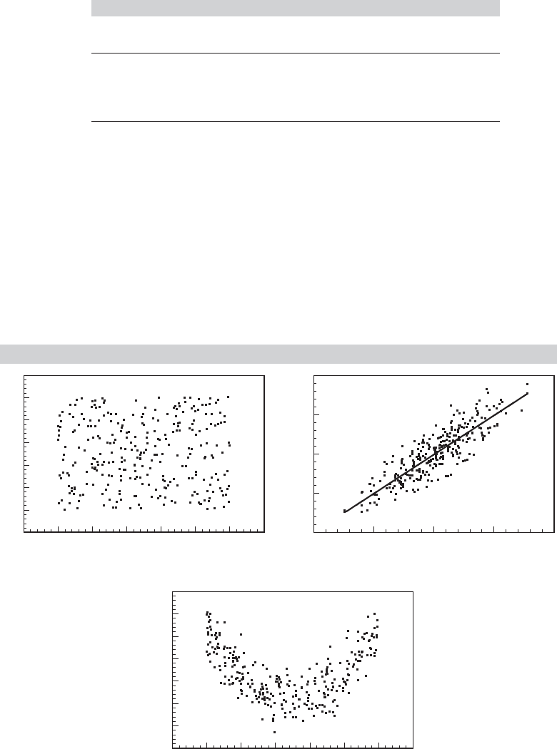
Figure 3.3 shows three possible cases for a simple linear regression model. The measure

of ﬁt described here embodies both the ﬁtting criterion and the covariation of y and x.

FIGURE 3.3

Sample Data.

1.2

1.0

.2

.2 .0 .2 .4 .6 .8 1.0 1.2

No Fit

2

4 2024

Moderate Fit

.8 1.0 1.2 1.4 1.6 1.8 2.0 2.2

.375

.300

.225

.150

.075

.000

.075

.150

No Fit

PART I

✦

The Linear Regression Model

, y

)

 y

 y¯

y¯

 y¯

 x¯

x¯

b(x

 x¯)

FIGURE 3.4

Decomposition of

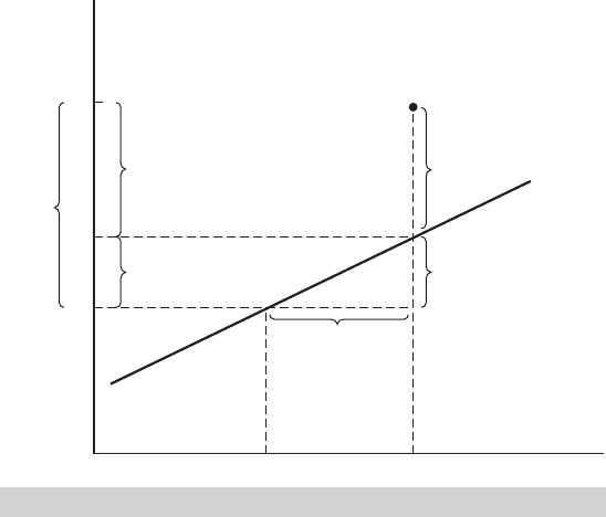
Variation of the dependent variable is deﬁned in terms of deviations from its mean,

− ¯y ).Thetotal variation in y is the sum of squared deviations:

SST =



i=1

− ¯y )

In terms of the regression equation, we may write the full set of observations as

y = Xb +e =

y + e.

For an individual observation, we have

= ˆy

+ e

= x



b + e

If the regression contains a constant term, then the residuals will sum to zero and the

mean of the predicted values of y

will equal the mean of the actual values. Subtracting

¯y from both sides and using this result and result 2 in Section 3.2.3 gives

− ¯y = ˆy

− ¯y + e

= (x

−



b + e

Figure 3.4 illustrates the computation for the two-variable regression. Intuitively, the

regression would appear to ﬁt well if the deviations of y from its mean are more largely

accounted for by deviations of x from its mean than by the residuals. Since both terms

in this decomposition sum to zero, to quantify this ﬁt, we use the sums of squares

instead. For the full set of observations, we have

y = M

Xb + M

where M

is the n × n idempotent matrix that transforms observations into deviations

from sample means. (See (3-21) and Section A.2.8.) The column of M

X corresponding

to the constant term is zero, and, since the residuals already have mean zero, M

e = e.

CHAPTER 3

✦

Least Squares

Then, since e



X = e



X = 0, the total sum of squares is



y = b



Xb + e



Write this as total sum of squares =regression sum of squares +error sum of squares, or

SST = SSR +SSE. (3-25)

(Note that this is the same partitioning that appears at the end of Section 3.2.4.)

We can now obtain a measure of how well the regression line ﬁts the data by

using the

coefﬁcient of determination:

SSR

SST



= 1 −



. (3-26)

The coefﬁcient of determination is denoted R

. As we have shown, it must be between

0 and 1, and it measures the proportion of the total variation in y that is accounted for

by variation in the regressors. It equals zero if the regression is a horizontal line, that

is, if all the elements of b except the constant term are zero. In this case, the predicted

values of y are always ¯y, so deviations of x from its mean do not translate into different

predictions for y. As such, x has no explanatory power. The other extreme, R

=1,

occurs if the values of x and y all lie in the same hyperplane (on a straight line for a

two variable regression) so that the residuals are all zero. If all the values of y

lie on a

vertical line, then R

has no meaning and cannot be computed.

Regression analysis is often used for forecasting. In this case, we are interested in

how well the regression model predicts movements in the dependent variable. With this

in mind, an equivalent way to compute R

is also useful. First



Xb =



but

y = Xb, y =

y + e, M

e = e, and X



e = 0, so



y =



y. Multiply



y/y



y =



y/y



y by 1 =



y to obtain

[

− ¯y)( ˆy

−

¯y)]

[

− ¯y)

][

( ˆy

−

¯y)

]

, (3-27)

which is the squared correlation between the observed values of y and the predictions

produced by the estimated regression equation.

Example 3.2 Fit of a Consumption Function

The data plotted in Figure 2.1 are listed in Appendix Table F2.1. For these data, where y is

C and x is X, we have ¯y = 273.2727, ¯x = 323.2727, S

= 12,618.182, S

= 12,300.182,

= 8,423.182 so SST = 12,618.182, b = 8,423.182/12,300.182 = 0.6848014, SSR =

= 5,768.2068, and SSE = SST − SSR = 6,849.975. Then R

= b

/SST =

0.457135. As can be seen in Figure 2.1, this is a moderate ﬁt, although it is not particu-

larly good for aggregate time-series data. On the other hand, it is clear that not accounting

for the anomalous wartime data has degraded the ﬁt of the model. This value is the R

for

the model indicated by the dotted line in the ﬁgure. By simply omitting the years 1942–1945

from the sample and doing these computations with the remaining seven observations—the

heavy solid line—we obtain an R

of 0.93697. Alternatively, by creating a variable WAR which

equals 1 in the years 1942–1945 and zero otherwise and including this in the model, which

produces the model shown by the two solid lines, the R

rises to 0.94639.

We can summarize the calculation of R

in an analysis of variance table, which

might appear as shown in Table 3.3.

PART I

✦

The Linear Regression Model

TABLE 3.3

Analysis of Variance

Source Degrees of Freedom Mean Square

Regression b



y − n ¯y

K − 1 (assuming a constant term)

Residual e



e n − Ks

Total y



y − n ¯y

n − 1 S

/(n − 1) = s

Coefﬁcient of R

= 1 −e



e/(y



y − n ¯y

)

determination

TABLE 3.4

Analysis of Variance for the Investment Equation

Source Degrees of Freedom Mean Square

Regression 0.0159025 4 0.003976

Residual 0.0004508 10 0.00004508

Total 0.016353 14 0.0011681

= 0.0159025/0.016353 = 0.97245

Example 3.3 Analysis of Variance for an Investment Equation

The analysis of variance table for the investment equation of Section 3.2.2 is given in

Table 3.4.

3.5.1 THE ADJUSTED

-SQUARED AND A MEASURE OF FIT

There are some problems with the use of R

in analyzing goodness of ﬁt. The ﬁrst

concerns the number of degrees of freedom used up in estimating the parameters.

[See (3-22) and Table 3.3] R

will never decrease when another variable is added to a

regression equation. Equation (3-23) provides a convenient means for us to establish

this result. Once again, we are comparing a regression of y on X with sum of squared

residuals e



e to a regression of y on X and an additional variable z, which produces sum

of squared residuals u



u. Recall the vectors of residuals z

∗

= Mz and y

∗

= My = e,

which implies that e



e = (y



∗

). Let c be the coefﬁcient on z in the longer regression.

Then c = (z



∗

)

−1



∗

), and inserting this in (3-24) produces



u = e



e −



∗

)



∗

)

= e





1 −r

∗2



, (3-28)

where r

∗

is the partial correlation between y and z, controlling for X. Now divide

through both sides of the equality by y



y. From (3-26), u



u/y



y is (1 − R

) for the

regression on X and z and e



e/y



y is (1 − R

). Rearranging the result produces the

following:

THEOREM 3.6

Change in R

When a Variable Is Added

to a Regression

Let R

be the coefﬁcient of determination in the regression of y on X and an

additional variable z, let R

be the same for the regression of y on X alone, and

let r

∗

be the partial correlation between y and z, controlling for X. Then

= R



1 − R



∗2

. (3-29)

CHAPTER 3

✦

Least Squares

Thus, the R

in the longer regression cannot be smaller. It is tempting to exploit

this result by just adding variables to the model; R

will continue to rise to its limit

of 1.

The adjusted R

(for degrees of freedom), which incorporates a penalty for these

results is computed as follows

= 1 −



e/(n − K)



y/(n − 1)

. (3-30)

For computational purposes, the connection between R

and

= 1 −

n − 1

n − K

(1 − R

The adjusted R

may decline when a variable is added to the set of independent variables.

Indeed,

may even be negative. To consider an admittedly extreme case, suppose that

x and y have a sample correlation of zero. Then the adjusted R

will equal −1/(n − 2).

[Thus, the name “adjusted R-squared” is a bit misleading—as can be seen in (3-30),

is not actually computed as the square of any quantity.] Whether

rises or falls

depends on whether the contribution of the new variable to the ﬁt of the regression

more than offsets the correction for the loss of an additional degree of freedom. The

general result (the proof of which is left as an exercise) is as follows.

THEOREM 3.7

Change in

When a Variable Is Added

to a Regression

In a multiple regression,

will fall (rise) when the variable x is deleted from the

regression if the square of the t ratio associated with this variable is greater (less)

than 1.

We have shown that R

will never fall when a variable is added to the regression.

We now consider this result more generally. The change in the residual sum of squares

when a set of variables X

is added to the regression is



1,2

= e



− b



where we use subscript 1 to indicate the regression based on X

alone and 1,2 to indicate

the use of both X

and X

. The coefﬁcient vector b

is the coefﬁcients on X

in the

multiple regression of y on X

and X

. [See (3-19) and (3-20) for deﬁnitions of b

and

.] Therefore,

1,2

= 1 −



− b



= R



This result comes at a cost, however. The parameter estimates become progressively less precise as we do

so. We will pursue this result in Chapter 4.

This measure is sometimes advocated on the basis of the unbiasedness of the two quantities in the fraction.

Since the ratio is not an unbiased estimator of any population quantity, it is difﬁcult to justify the adjustment

on this basis.

PART I

✦

The Linear Regression Model

which is greater than R

unless b

equals zero. (M

could not be zero unless X

was a

linear function of X

, in which case the regression on X

and X

could not be computed.)

This equation can be manipulated a bit further to obtain

1,2

= R



But y



y = e



, so the ﬁrst term in the product is 1 − R

. The second is the multiple

correlation in the regression of M

y on M

, or the partial correlation (after the effect

of X

is removed) in the regression of y on X

. Collecting terms, we have

1,2

= R



1 − R



y2·1

[This is the multivariate counterpart to (3-29).]

Therefore, it is possible to push R

as high as desired just by adding regressors.

This possibility motivates the use of the adjusted R

in (3-30), instead of R

as a

method of choosing among alternative models. Since

incorporates a penalty for

reducing the degrees of freedom while still revealing an improvement in ﬁt, one pos-

sibility is to choose the speciﬁcation that maximizes

. It has been suggested that

the adjusted R

does not penalize the loss of degrees of freedom heavily enough.

Some alternatives that have been proposed for comparing models (which we index

by j ) are

= 1 −

n + K

n − K



1 − R



which minimizes Amemiya’s (1985) prediction criterion,



n − K



1 +



= s



1 +



and the Akaike and Bayesian information criteria which are given in (5-43) and

(5-44).

3.5.2

-SQUARED AND THE CONSTANT TERM IN THE MODEL

A second difﬁculty with R

concerns the constant term in the model. The proof that

0 ≤ R

≤1 requires X to contain a column of 1s. If not, then (1) M

e =e and

(2) e



X = 0, and the term 2e



Xb in y



y = (M

Xb + M



Xb + M

in the expansion preceding (3-25) will not drop out. Consequently, when we compute

= 1 −



the result is unpredictable. It will never be higher and can be far lower than the same

ﬁgure computed for the regression with a constant term included. It can even be negative.

See, for example, Amemiya (1985, pp. 50–51).

Most authors and computer programs report the logs of these prediction criteria.

CHAPTER 3

✦

Least Squares

Computer packages differ in their computation of R

. An alternative computation,



is equally problematic. Again, this calculation will differ from the one obtained with the

constant term included; this time, R

may be larger than 1. Some computer packages

bypass these difﬁculties by reporting a third “R

,” the squared sample correlation be-

tween the actual values of y and the ﬁtted values from the regression. This approach

could be deceptive. If the regression contains a constant term, then, as we have seen, all

three computations give the same answer. Even if not, this last one will still produce a

value between zero and one. But, it is not a proportion of variation explained. On the

other hand, for the purpose of comparing models, this squared correlation might well be

a useful descriptive device. It is important for users of computer packages to be aware

of how the reported R

is computed. Indeed, some packages will give a warning in the

results when a regression is ﬁt without a constant or by some technique other than linear

least squares.

3.5.3 COMPARING MODELS

The value of R

of 0.94639 that we obtained for the consumption function in Ex-

ample 3.2 seems high in an absolute sense. Is it? Unfortunately, there is no absolute

basis for comparison. In fact, in using aggregate time-series data, coefﬁcients of deter-

mination this high are routine. In terms of the values one normally encounters in cross

sections, an R

of 0.5 is relatively high. Coefﬁcients of determination in cross sections

of individual data as high as 0.2 are sometimes noteworthy. The point of this discussion

is that whether a regression line provides a good ﬁt to a body of data depends on the

setting.

Little can be said about the relative quality of ﬁts of regression lines in different

contexts or in different data sets even if they are supposedly generated by the same data

generating mechanism. One must be careful, however, even in a single context, to be

sure to use the same basis for comparison for competing models. Usually, this concern

is about how the dependent variable is computed. For example, a perennial question

concerns whether a linear or loglinear model ﬁts the data better. Unfortunately, the

question cannot be answered with a direct comparison. An R

for the linear regression

model is different from an R

for the loglinear model. Variation in y is different from

variation in ln y. The latter R

will typically be larger, but this does not imply that the

loglinear model is a better ﬁt in some absolute sense.

It is worth emphasizing that R

is a measure of linear association between x and y.

For example, the third panel of Figure 3.3 shows data that might arise from the model

= α + β(x

− γ)

+ ε

(The constant γ allows x to be distributed about some value other than zero.) The

relationship between y and x in this model is nonlinear, and a linear regression would

ﬁnd no ﬁt.

A ﬁnal word of caution is in order. The interpretation of R

as a proportion of

variation explained is dependent on the use of least squares to compute the ﬁtted

PART I

✦

The Linear Regression Model

values. It is always correct to write

− ¯y = ( ˆy

− ¯y) + e

regardless of how ˆy

is computed. Thus, one might use ˆy

= exp(



lny

) from a loglinear

model in computing the sum of squares on the two sides, however, the cross-product

term vanishes only if least squares is used to compute the ﬁtted values and if the model

contains a constant term. Thus, the cross-product term has been ignored in computing

for the loglinear model. Only in the case of least squares applied to a linear equation

with a constant term can R

be interpreted as the proportion of variation in y explained

by variation in x. An analogous computation can be done without computing deviations

from means if the regression does not contain a constant term. Other purely algebraic

artifacts will crop up in regressions without a constant, however. For example, the value

of R

will change when the same constant is added to each observation on y, but it

is obvious that nothing fundamental has changed in the regression relationship. One

should be wary (even skeptical) in the calculation and interpretation of ﬁt measures for

regressions without constant terms.

3.6 LINEARLY TRANSFORMED REGRESSION

As a ﬁnal application of the tools developed in this chapter, we examine a purely alge-

braic result that is very useful for understanding the computation of linear regression

models. In the regression of y on X, suppose the columns of X are linearly transformed.

Common applications would include changes in the units of measurement, say by chang-

ing units of currency, hours to minutes, or distances in miles to kilometers. Example 3.4

suggests a slightly more involved case.

Example 3.4 Art Appreciation

Theory 1 of the determination of the auction prices of Monet paintings holds that the price

is determined by the dimensions (width, W and height, H) of the painting,

ln P = β

(1) + β

ln W + β

ln H + ε

= β

+ β

+ ε.

Theory 2 claims, instead, that art buyers are interested speciﬁcally in surface area and aspect

ratio,

ln P = γ

(1) + γ

ln(WH) + γ

ln(W/H) + ε

= γ

+ γ

+ u.

It is evident that z

= x

, z

= x

+ x

and z

= x

− x

. In matrix terms, Z = XP where

P =



10 0

01 1

01−1



The effect of a transformation on the linear regression of y on X compared to that

of y on Z is given by Theorem 3.8.

CHAPTER 3

✦

Least Squares

THEOREM 3.8

Transformed Variables

In the linear regression of y on Z = XP where P is a nonsingular matrix that

transforms the columns of X, the coefﬁcients will equal P

−1

b where b is the vector

of coefﬁcients in the linear regression of y on X, and the R

will be identical.

Proof: The coefﬁcients are

d = (Z



−1



y = [(XP)



(XP)]

−1

(XP)



y = (P



XP)

−1



= P

−1



−1

−1



y = P

−1

The vector of residuals is u = y−Z(P

−1

b) = y−XPP

−1

b = y−Xb = e. Since the

residuals are identical, the numerator of 1− R

is the same, and the denominator

is unchanged. This establishes the result.

This is a useful practical, algebraic result. For example, it simpliﬁes the analysis in the

ﬁrst application suggested, changing the units of measurement. If an independent vari-

able is scaled by a constant, p, the regression coefﬁcient will be scaled by 1/p. There is

no need to recompute the regression.

3.7 SUMMARY AND CONCLUSIONS

This chapter has described the purely algebraic exercise of ﬁtting a line (hyperplane) to a

set of points using the method of least squares. We considered the primary problem ﬁrst,

using a data set of n observations on K variables. We then examined several aspects of

the solution, including the nature of the projection and residual maker matrices and sev-

eral useful algebraic results relating to the computation of the residuals and their sum of

squares. We also examined the difference between gross or simple regression and corre-

lation and multiple regression by deﬁning “partial regression coefﬁcients” and “partial

correlation coefﬁcients.” The Frisch–Waugh–Lovell theorem (3.2) is a fundamentally

useful tool in regression analysis that enables us to obtain in closed form the expres-

sion for a subvector of a vector of regression coefﬁcients. We examined several aspects

of the partitioned regression, including how the ﬁt of the regression model changes

when variables are added to it or removed from it. Finally, we took a closer look at the

conventional measure of how well the ﬁtted regression line predicts or “ﬁts” the data.

Key Terms and Concepts

•

Adjusted R

•

Analysis of variance

•

Bivariate regression

•

Coefﬁcient of determination

•

Degrees of Freedom

•

Disturbance

•

Fitting criterion

•

Frisch–Waugh theorem

•

Goodness of ﬁt

•

Least squares

•

Least squares normal

equations

•

Moment matrix

•

Multiple correlation

•

Multiple regression

•

Netting out

•

Normal equations

•

Orthogonal regression

•

Partial correlation

coefﬁcient

•

Partial regression coefﬁcient

PART I

✦

The Linear Regression Model

•

Partialing out

•

Partitioned regression

•

Prediction criterion

•

Population quantity

•

Population regression

•

Projection

•

Projection matrix

•

Residual

•

Residual maker

•

Total variation

Exercises

1. The two variable regression. For the regression model y = α + βx + ε,

a. Show that the least squares normal equations imply 

= 0 and 

= 0.

b. Show that the solution for the constant term is a = ¯y − b ¯x.

c. Show that the solution for b is b = [



i=1

− ¯x)(y

− ¯y)]/[



i=1

− ¯x)

d. Prove that these two values uniquely minimize the sum of squares by showing

that the diagonal elements of the second derivatives matrix of the sum of squares

with respect to the parameters are both positive and that the determinant is

4n[(



i=1

) − n ¯x

] = 4n[



i=1

− ¯x )

], which is positive unless all values of

x are the same.

2. Change in the sum of squares. Suppose that b is the least squares coefﬁcient vector

in the regression of y on X and that c is any other K × 1 vector. Prove that the

difference in the two sums of squared residuals is

(y − Xc)



(y − Xc) − (y − Xb)



(y − Xb) = (c −b)



X(c − b).

Prove that this difference is positive.

3. Partial Frisch and Waugh. In the least squares regression of y on a constant and X,

to compute the regression coefﬁcients on X, we can ﬁrst transform y to deviations

from the mean ¯y and, likewise, transform each column of X to deviations from the

respective column mean; second, regress the transformed y on the transformed X

without a constant. Do we get the same result if we only transform y? What if we

only transform X?

4. Residual makers. What is the result of the matrix product M

M where M

is deﬁned

in (3-19) and M is deﬁned in (3-14)?

5. Adding an observation. A data set consists of n observations on X

and y

. The least

squares estimator based on these n observations is b

= (X



)

−1



. Another

observation, x

and y

, becomes available. Prove that the least squares estimator

computed using this additional observation is

n,s

= b

1 + x



)

−1



)

−1

− x



Note that the last term is e

, the residual from the prediction of y

using the coefﬁ-

cients based on X

and b

. Conclude that the new data change the results of least

squares only if the new observation on y cannot be perfectly predicted using the

information already in hand.

6. Deleting an observation. A common strategy for handling a case in which an ob-

servation is missing data for one or more variables is to ﬁll those missing variables

with 0s and add a variable to the model that takes the value 1 for that one ob-

servation and 0 for all other observations. Show that this “strategy” is equivalent

to discarding the observation as regards the computation of b but it does have an

effect on R

. Consider the special case in which X contains only a constant and one